EXCEL Output and Drawing upon Statistical Procedures - Dissertation Example

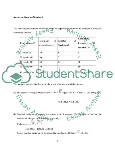
EXCEL Output and Drawing upon Statistical Procedures Answer to Question Number 1 The following table shows the details about the expenditure on books by a sample of first year economics students. Expenditure (£) Mid-point of expenditure (x) Number of Students (f) Cumulative frequency of students (F) 0 – under 20 10 6 6 20 – under 40 30 7 13 40 – under 60 50 25 38 60 – under 80 70 12 50 80 – under 120 100 8 58 (= N = ) The required statistics in reference to the above table, are provided as under – (a) The mean of the expenditures on books, X* =  = [(6 x 10) + (7 x 30) + … (8 x 100)] /58 = £ 54.4828 ≈ £ 54.48. (b) Standard deviation is actually the square root of variance. The formula to find out the variance of a frequency distribution is given by, Variance = s2 = -  = 3589.66 – 2968.37 = 621.28 Hence, standard deviation on the expenditure on books, SD (x) =  = 24.93. (c) The formula for median in case of grouped data is given by, M =. Where, n = Number of observations in the sample, F = Cumulative Distribution till the median class. f = Frequency at the median class. W = Median class width and Lm = Lower boundary of the median class. The median class is that which contains the (n/2)th observation. Here, n = 58, so, n/2 = 29. Thus the median class in this case is, (40 – under 60) since the cumulative distribution of that class is 38, while that of its previous class is 9. Hence, here, F = 9, f = 25, w = 20 and Lm = 40. Therefore, median, M =  = 56 (£). (d) The null hypothesis to be tested in this case is as follows, H0: µ = 55.23 against the alternative hypothesis, H1: µ ≠ 55.23. It is clear from the form of the alternative hypothesis that the test is a two-tailed one. The sample mean is found to be 54.48 The population standard deviation is again reported as, σ = 16. The appropriate test statistic for testing the consistency of population mean for large samples (n > 30) is the z-statistic, which is defined as, Z =  =  = 0.0469. The estimated z-statistic has to be compared with the tabulated value of z at 95% confidence interval. Since the present case is that of a two-tailed test, so, the value of tabulated z-statistic at 5% level of significance is, Z0.025 = 1.96. Clearly, tabulated | Z | < Z0.025. Hence, the null hypothesis cannot be rejected at 5% level of significance, implying that in 95% of the cases, the population mean is found not to be significantly different from £ 55.23. Answer to Question Number 2 The values for R and S have been specified in the above case as, R = 6 and S = 8 respectively. It is given that the values of aggregate investment (I) in the economy for the following year are predicted to follow normal distribution with mean, 146 (140 + R) and standard deviation, 8 (= S). The list of 50 such random numbers that the aggregate investment is expected to take, is presented in the appendix of the paper (Appendix A.1: List of Random Numbers). (a) Descriptive statistics are meant to explain the main characteristics of a collection of raw data in quantitative terms. The purpose of descriptive statistics is to give a placid view about the sample under consideration. Some of the most important descriptive statistics that help to judge the main features of a sample are - mean, median, standard deviation, range and the inter-quartile range. The mean and median are three different measures of central tendency for a given set of data. Mean is most suitable in case of ungrouped data or in cases where the data does not have a frequency distribution. On the other hand, median measures the middlemost value of the sample after the data has been arranged in an ascending order. However, the two measures yield almost similar results in cases of ungrouped data, since any central tendency statistic in such cases is aimed at finding the average value from all observations. In the present case, the mean and the median statistics for the 50 observations of random variables are expected to be almost similar since there is no scope for repetition of values in this case. The formula for mean is, x =  ∑ x2, while, The median observation could be found by arranging all the observations in an ascending order and then by implementing the formula, M = 0.5 x (n + 1). (Here n implies the number of sample observations). Standard deviation, range and inter-quartile range, on the other hand are three different measures of dispersion of the sample observations. Measures of dispersion are meant to estimate the degree of variation present in a given sample. Standard deviation however is considered to be a better measure of the same than range, which in fact is considered as a rather primitive measure. However, inter-quartile range, although not used extensively, can rather be considered as a more reliable measure of dispersion that considers the difference between the 75th and the 25th percentiles in the given dataset. The formula to find standard deviation is, σ = ^2. On the other hand, to find range, one has to sort the data in an ascending order and find out the maximum and minimum values from the observations. The formula to find out the range of the given dataset is, Range = (Maximum – Minimum). The method to find out the inter-quartile range is, first arrange the dataset in an ascending order and then find out the observations positioned at the 75% and 25% points respectively. Then calculate inter-quartile range as, Q3 – Q1. The descriptive statistics mentioned above for the given set of random variables is presented as under - Mean 145.5856 Median 146.11316 Standard Deviation 6.8409959 Minimum 129.75393 Maximum 161.24069 Range 31.486768 25th percentile 139.7326452 75th percentile 149.447209 Inter-quartile range 9.7145638 (b) The cumulative frequency table, histogram and polygon for the given set of random sample observations for aggregate investment is provided as under – Cumulative Frequency Distribution Table It shows the cumulative number of observations in a given class interval, i.e., how the frequency of the various class intervals keep on rising as the number of classes increase. On the other hand, cumulative frequency percentage is that which shows the percentage of observations being covered till a particular class is reached, so that at the last class interval, exactly 100% of the observations are covered. Class Intervals Frequency Cumulative Frequency Cumulative % 120.00 – 124.99 0 0 0.00% 125.00 – 129.99 1 1 2.00% 130.00 – 134.99 1 2 4.00% 135.00 – 139.99 10 12 24.00% 140.00 – 144.99 9 21 42.00% 145.00 – 149.99 17 38 76.00% 150.00 – 154.99 9 47 94.00% 155.00 – 159.99 0 47 94.00% 160.00 – 164.99 3 50 100.00% More 0 50 100.00% Histogram Histogram is a graphical representation showing the frequency distribution for a particular class interval, for a given set of data, in the form of bars representing the frequencies for each class. It shows the proportion of total observations that fall within each class interval. In the diagram below, the histogram is found to exhibit cumulative frequencies in quantity as well as a cumulative percentage. Frequency Polygon Frequency polygon is similar to a histogram, with the only difference that the frequencies for each class are connected with one another with the help of a line, in a chart. The frequency polygon provides information about the nature of the distribution of the observations. It serves the same purpose as a histogram from this aspect, but the former is able to find out the underlying frequency distribution in a more clarified way. From the frequency polygon plot shown below, it is evident that the random numbers being chosen as tentative values of aggregate investment for the following year display a normal distribution curve. (c) The features of aggregate investment for the following year, based on the assumption that the values are normally distributed, has been explained with the help of descriptive statistics as has been provided under. The mean of all random values that aggregate investment is expected to take, is found to be 145.5856, while the median is 146.11316. It is thus obvious that there is not much difference; or rather the difference is very insignificant, between the two measures of central tendency. This fact is obvious given that the underlying random variables being extracted, with mean and standard deviation of the past values that aggregate investment has taken has been considered to be random in nature. On the other hand, the higher the measures of dispersion within the dataset, higher will be the degree of variability within the observations. In the present case it is noticed that, the standard deviation is 6.8409959, the range of the observations is 31.486768, while the value of the inter-quartile measure of dispersion is 9.7145638. The standard deviation is the most reliable measure of standard deviation, the second-most reliable in the present case is the inter-quartile range and the least reliable is range. The reliability of range is minimum, since it considers the difference between the highest and the lowest numbers in a dataset. If now, the minimum is too low with all other observations lying near to one another or the maximum is posited very high with all other observations quite low and lying almost in a uniform manner, the range hence measured will be very high, even though the overall degree of variation might not be so. This is the reason why this particular measure of dispersion is the most unreliable one. Hence, the value of the statistic in the present case (31.486768) is not being considered in a serious way; rather the two other statistics are being treated with greater importance. The inter-quartile range is important since almost 67% of the total observations are supposed to lie within this range, in case of a normal distribution and thus it is able to consider a high number of observations for any analysis. This statistic is found to be almost equal with the standard deviation of the given dataset. This factor suggests that the variations in the tentative observations cannot be less than 6.8409959, but cannot be more than 9.7145638 as well. However, since the former is a far more reliable measure, so, it is preferred to the latter value in order to decide the range of the values that the aggregate investment in the following year is supposed to take. Hence, arbitrarily it can be said that the value of aggregate observations will be lying within a range of (6.84 ± 145.5856) = (138.7446, 152.4266) Answer to Question Number 3 (a) The relationship between Income (Y), Inflation (P0), Unemployment (U) and Social Welfare (SW) are provided as under – U = %, P0 = % and SW = . Here, R = 6 and S = 8 has already been specified previously. Hence, the values of the variables Inflation and Unemployment for given values of Income are presented as under – The above values suggest that there is more or less an inverse relationship between the rates of inflation and unemployment. It is observed that higher the rate of inflation goes, lower becomes the rate of unemployment. On the contrary, lower the rate of inflation is, higher is the rate of unemployment present in the economy. This is in compliance with economic theory since, lower the rate of inflation in an economy is, lower will be the general price level in the nation, thus hampering the market price of the commodities. Thus there arises a scope for producer loss and then they start holding back the commodities already produced and temporarily cut down their production capacities, so as to raise the market price of the goods. In the process of cutting down productive capacity, the employers start retrenching any additional labour once employed to enhance the production capacity. Thus, lower inflation is always associated with a low rate of unemployment and vice versa. (b) The following represents a closed economy Y =C + I + G C =a + (b x YD) YD = Y - T T = t x Y Where Y = Income, I = Investment, G = Government Spending, C = Consumption YD = Disposable Income. T = Taxes, and a, b, t are parameters, with a = 5 and b = 0.85. The value of b is nothing but the marginal propensity to consume. Higher this amount gets, lower will be the savings in the economy and lower will be any scope for future investment. The investment for the following year is 142.5 (i) When the tax rate is 0.4 and government spending is 50, then T = 0.4Y, YD = Y – 0.4Y = 0.6Y. Consumption, C = 5 + (0.85 x 0.6Y) = 5 + 0.51Y. Hence, income, Y = 5 + 0.51 Y + 142.5 + 50 0.51 Y = 197.5 Y = 403.0612. (ii) When tax rate (t) is 0.22 and government spending (G) is 50, then, T = 0.22Y, YD = Y – 0.22Y = 0.78Y. Consumption, C = 5 + (0.85 x 0.78Y) = 5 + 0.663Y. Hence, income, Y = 5 + 0.663 Y + 142.5 + 50 0.663 Y = 197.5 Y = 297.89. (iii) When tax rate (t) is 0.24 and government spending (G) is 150, then, T = 0.24Y, YD = Y – 0.24Y = 0.76Y. Consumption, C = 5 + (0.85 x 0.76Y) = 5 + 0.646Y. Hence, income, Y = 5 + 0.646 Y + 142.5 + 150 0.646 Y = 297.5 Y = 460.53. Thus it is found that the government would be in the most advantageous position if it follows the third strategy. Hence, the third situation is the most desirable one. Bibliography Mankiw, N. G. (2003) Macroeconomics (9th Edition). New York: Worth Publishers. Appendix: List of Random Numbers 148.5297 161.2407 152.1448 148.1337 150.4654 143.0859 139.3057 160.3572 135.0277 142.4407 146.1548 160.5898 147.7455 151.3408 138.5794 135.2796 135.4832 148.8948 154.771 145.6414 143.4887 143.8372 138.5895 135.4701 146.5796 147.9642 147.128 146.0479 144.6309 138.7994 134.2018 129.7539 152.8315 150.1253 146.1284 143.4799 146.0979 149.9997 144.5771 142.7288 140.0352 138.2194 148.6626 152.7732 145.5762 139.4301 151.8815 147.1688 151.6123 146.2495 Read More