Analyzing the Year of Studying - Assignment Example

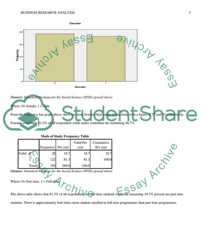
Business Research Analysis (i) Describe the following data using appropriate graphical displays and summary statistics: year of study, gender, number of hours used per week, overall satisfaction and the three satisfaction ratings for stock, quiet areas and staff. Use your results to provide a summary of these issues, highlighting potential areas for improvement. Descriptive Statistics N Range Minimum Maximum Mean Std. Deviation Variance Statistic Statistic Statistic Statistic Statistic Std. Error Statistic Statistic Age 150 26 18 44 21.73 .274 3.359 11.284 Year 150 4 4 8 5.62 .093 1.145 1.311 Hours 150 25 0 25 12.47 .561 6.875 47.271 Stock 150 8 2 10 6.01 .205 2.510 6.302 Quiet 150 8 2 10 6.43 .181 2.221 4.931 Staff 150 7 3 10 7.00 .109 1.331 1.772 Satisfaction 150 91 5 96 55.22 1.740 21.305 453.918 Valid N (list-wise) 150 (Source: Statistical Package for the Social Science (SPSS) spread sheet) There are a total number of 150 respondents in this study. From the above table, the mean age of the respondents is 21.73 years with a minimum of 18 and a maximum of 44 years. A notable characteristic of the three satisfaction ratings for stock, quiet areas and staff is above average mean ratings. Gender Frequency Bar Graph (Source: Statistical Package for the Social Science (SPSS) spread sheet) Where: 0= female, 1 = male From the frequency bar graph above, there are more females than males in the study with a figure of 77 and 73 respectively. Females contribute 51.3% of all respondent while males contribute the remaining 48.7%. Mode of Study Frequency Table Frequency Per cent Valid Per cent Cumulative Per cent Valid 0 28 18.7 18.7 18.7 1 122 81.3 81.3 100.0 Total 150 100.0 100.0 (Source: Statistical Package for the Social Science (SPSS) spread sheet) Where: 0= Part time, 1 = Full time The above table shows that 81.3% of all respondents are full time students while the remaining 18.7% percent are part time students. There is approximately four times more student enrolled in full time programmes than part time programmes. Year of Study Frequency Bar Graph (Source: Statistical Package for the Social Science (SPSS) spread sheet) Where: 4 = Year 1 Undergraduate 5 = Year 2 Undergraduate 6 = Year 3 Undergraduate (Final Year) 7 = Postgraduate (e.g. MBA, MSc) 8 = Doctoral (e.g. PhD) The above graph shows that the number of respondents increase from the first year to the fifth year of undergraduate studies after which it decrease towards the doctoral level of study. (Source: Statistical Package for the Social Science (SPSS) spread sheet) Age of respondents ranges from 18 to 44 years. Respondents of 18 years of age are the majority in the sample. Respondents of 27, 28, 33, 35 and 44 years form the minority each contributing 0.7% of the respondents. Potential Areas for Improvement From the gender frequency bar, it is clear that the number of female respondents exceed that of their male counterparts. From majority of statistics, majority of tertiary education students are male. The following sample should have used a controlled number of male and female respondents which reflect the actual gender proportions of the parent population. The number of sampled full time students is also too many compared to part time students. The number of sampled respondents who are more than 27 years of age is too little those with less than 25 years. These biases should be reduced in order to ensure that the sampled population reflects the characteristics of the parent population as closely as possible. (ii) To what extent is there a difference of opinion between males and females relating to the three satisfaction ratings for stock, quiet areas and staff? We will use the independent sample t-test since it shows whether there is a significant difference between the means of two groups of people or conditions. Group Statistics Gender N Mean Std. Deviation Std. Error Mean Stock 0 77 5.84 2.444 .279 1 73 6.18 2.584 .302 Quiet 0 77 6.53 2.174 .248 1 73 6.32 2.278 .267 Staff 0 77 6.97 1.224 .140 1 73 7.03 1.443 .169 (Source: Statistical Package for the Social Science (SPSS) spread sheet) From the above, we see that there are more female respondents than male respondents in the three satisfaction rations. The means of males and females in three satisfaction rations differ. The table below analyses this mean differences. Independent Samples Test Levenes Test for Equality of Variances t-test for Equality of Means F Sig. t df Sig. (2-tailed) Mean Difference Std. Error Difference 95% Confidence Interval of the Difference Lower Upper Stock Equal variances assumed .882 .349 -.813 148 .417 -.334 .411 -1.145 .477 Equal variances not assumed -.812 146.262 .418 -.334 .411 -1.147 .479 Quiet Equal variances assumed .492 .484 .598 148 .551 .217 .364 -.501 .936 Equal variances not assumed .597 146.519 .551 .217 .364 -.502 .937 Staff Equal variances assumed 1.115 .293 -.245 148 .807 -.053 .218 -.484 .378 Equal variances not assumed -.244 141.415 .808 -.053 .219 -.486 .380 (Source: Statistical Package for the Social Science (SPSS) spread sheet) In the Independent Samples Test table above, the first part shows the Levenes Test for Equality of Variances. One of the assumptions of the t-test is the homogeneity of variance. Since the significance level (in the Levenes Test for Equality of Variances column) is greater than 0.05 for each of the three satisfaction rations, the assumption of homogeneity of variance is met. We will therefore use the ‘Equal variances assumed’ row to determine whether there is a significant difference between males and females satisfaction ratings. The null hypotheses can now be stated as: 1. There is no significant difference of opinion between males and females relating to the satisfaction ratings for stock. 2. There is no significant difference of opinion between males and females relating to the satisfaction ratings for quiet. 3. There is no significant difference of opinion between males and females relating to the satisfaction ratings for staff. All the figure in the ‘Sig. (2-tailed)’ column under the t-test for Equality of Means section are greater than 0.05. Therefore, we accept the three null hypotheses above. Managerial Implications It can now be concluded that the satisfaction ratings for stock, quiet and staff are not significantly different for male and female respondents. This means that both genders have approximately equal views on the three satisfaction ratings. If there was a significant difference between the mean ratings, there would be for affirmative action since it would imply that there is unfair treatment of female students. (iii) To what extent is there a difference between the modes of study and the number of hours spent in the library per week? We will use the independent sample t-test since it shows whether there is a significant difference between the means of two groups of people or conditions. Group Statistics Mode N Mean Std. Deviation Std. Error Mean Hours 0 28 9.29 3.029 .572 1 122 13.20 7.299 .661 Key: Study mode (0=Part time, 1= Full time) (Source: Statistical Package for the Social Science (SPSS) spread sheet) From the above table, there were 28 part time students who were sampled. They spent a mean number of 9.29 hours in the library per week. There were also 122 full time students who were sampled. They spent a mean number of 13.20 hours in the library per week. Independent Samples Test Levenes Test for Equality of Variances t-test for Equality of Means F Sig. t df Sig. (2-tailed) Mean Difference Std. Error Difference 95% Confidence Interval of the Difference Lower Upper Hours Equal variances assumed 29.019 .000 -2.781 148 .006 -3.919 1.409 -6.704 -1.134 Equal variances not assumed -4.483 105.216 .000 -3.919 .874 -5.653 -2.186 (Source: Statistical Package for the Social Science (SPSS) spread sheet) Since the significance level (in the Levenes Test for Equality of Variances column) is lower than 0.05, the assumption of homogeneity of variance is not met. We will therefore use the ‘Equal variances not assumed’ row to determine whether there is a significant difference between the modes of study and the number of hours spent in the library per week The null hypotheses can now be stated as: There is no significant difference of opinion between the modes of study and the number of hours spent in the library per week The figure in the ‘Sig. (2-tailed)’ column under the t-test for Equality of Means section is lower than 0.05. Therefore, we reject the null hypotheses above. Managerial Implication The above results show that the full time students significantly spend more hours in the library compared to part time student with the mean number of hours being of 9.29 hours for part time students and 13.20 hours for full time students. This may be so since part time students usually share their time between school and other activities. (iv) Investigate whether there are any differences in the overall satisfaction rating according to the year of study. Null Hypothesis: There are no differences in the overall satisfaction rating according to the year of study Alternative Hypothesis: There is at least one difference in the overall satisfaction rating according to the year of study We shall use the One-Way Analysis of Variance because it tests the equality of three or more means at one time by using variances Descriptives Satisfaction N Mean Std. Deviation Std. Error 95% Confidence Interval for Mean Minimum Maximum Year Lower Bound Upper Bound 4 28 67.86 15.427 2.915 61.88 73.84 44 96 5 46 55.74 15.056 2.220 51.27 60.21 30 80 6 38 71.79 5.846 .948 69.87 73.71 62 81 7 31 27.81 15.696 2.819 22.05 33.56 5 55 8 7 32.71 9.945 3.759 23.52 41.91 20 48 Total 150 55.22 21.305 1.740 51.78 58.66 5 96 (Source: Statistical Package for the Social Science (SPSS) spread sheet) Key: Year of study (4,5,6,7,8) Where 4 = Year 1 Undergraduate 5 = Year 2 Undergraduate 6 = Year 3 Undergraduate (Final Year) 7 = Postgraduate (e.g. MBA, MSc) 8 = Doctoral (e.g. PhD) The above table shows the number of respondents in each their respective years of study and the mean overall satisfaction rating Test of Homogeneity of Variances Satisfaction Levene Statistic df1 df2 Sig. 9.253 4 145 .000 (Source: Statistical Package for the Social Science (SPSS) spread sheet) The significance level in the above table is less than 0.05 meaning that the assumption of Homogeneity of Variances is violated. We will therefore employ the table labeled Robust Tests of Equality of Means as opposed to the Anova table. (Source: Statistical Package for the Social Science (SPSS) spread sheet) The significance value is less than 0.05 and thus, we reject the null hypothesis and go with the alternative hypothesis that there is at least one difference in the overall satisfaction rating according to the year of study. The above results do not show which group is different from the other. We will use the multiple comparisons table to determine this. Since the equality of variance was violated, we will interpret the results using the Games-Howell test (instead of Tukey HSD test) in the multiple comparisons table. From the multiple comparisons table below, the values with asterisks in the column labelled Mean Difference (I-J) shows groups with significant differences in their mean overall satisfaction rating. Multiple Comparisons Dependent Variable: Satisfaction (I) Year (J) Year Mean Difference (I-J) Std. Error Sig. 95% Confidence Interval Lower Bound Upper Bound Games-Howell 4 5 12.118* 3.664 .014 1.79 22.45 6 -3.932 3.066 .703 -12.78 4.91 7 40.051* 4.055 .000 28.62 51.48 8 35.143* 4.757 .000 20.35 49.93 5 4 -12.118* 3.664 .014 -22.45 -1.79 6 -16.050* 2.414 .000 -22.84 -9.26 7 27.933* 3.588 .000 17.85 38.01 8 23.025* 4.365 .002 8.85 37.20 6 4 3.932 3.066 .703 -4.91 12.78 5 16.050* 2.414 .000 9.26 22.84 7 43.983* 2.974 .000 35.45 52.51 8 39.075* 3.877 .000 25.08 53.07 7 4 -40.051* 4.055 .000 -51.48 -28.62 5 -27.933* 3.588 .000 -38.01 -17.85 6 -43.983* 2.974 .000 -52.51 -35.45 8 -4.908 4.699 .831 -19.58 9.76 8 4 -35.143* 4.757 .000 -49.93 -20.35 5 -23.025* 4.365 .002 -37.20 -8.85 6 -39.075* 3.877 .000 -53.07 -25.08 7 4.908 4.699 .831 -9.76 19.58 *. The mean difference is significant at the 0.05 level. (Source: Statistical Package for the Social Science (SPSS) spread sheet) Managerial Implication There is a significant difference in the overall satisfaction rating between first year students and all other groups except third year students. There is a significant difference in the overall satisfaction rating between second year students and all other groups. There is a significant difference in the overall satisfaction rating between third year students and all other groups except first year students. There is a significant difference in the overall satisfaction rating between postgraduate students and all other groups except doctoral students. There is a significant difference in the overall satisfaction rating between doctoral students and all other groups except postgraduate students. (v) Using appropriate graphical displays and statistical measures assess the extent to which the overall satisfaction is associated with the three rating scores for stock, quiet areas and staff. Pearson Moment Correlation will determine the extent to which the overall satisfaction is associated with the three quantitative rating scores for stock, quiet areas and staff. (Source: Statistical Package for the Social Science (SPSS) spread sheet) Managerial Implication From the correlation table above, the overall satisfaction positively related to the three rating scores for stock, quiet areas and staff. As the rating level for stock increases, the overall satisfaction increases. This is a statistically significant relationship as indicated by the significance level of 0.000 which is below is 0.05 level. As the rating level for staff increases, the overall satisfaction increases. This is a statistically significant relationship as indicated by the significance level of 0.000 which is below is 0.05 level. As the rating level for library quiet study areas increases, the overall satisfaction increase. This is not a statistically significant relationship as indicated by the significance level of 0.210 which is above is 0.05 level. From the correlation coefficient, the strongest relationship exists between satisfaction and stock rating since its value (0.886) is the closest to the absolute value of 1. Betterment of the resources in the library (Stock) would best improve the overall satisfaction rating by the students. This is well displays in the following Scatterplots which are forming a shape from the bottom left to the top right. This indicates a strong positive relationship just as proved by the correlation table. Scatterplots: Stock vs. Satisfaction (Source: Excel 2010) (vi) Using the best of the three predictors from the previous section, develop and interpret a simple regression model to predict overall satisfaction. Consider the following two cases: • One who gives scores of 3, 5 and 8 for stock, quiet areas and staff respectively • One who gives scores of 9, 10 and 7 for stock, quiet areas and staff respectively Use your regression model to predict their likely overall score and comment critically on the predictions made. The best predictor of overall satisfaction is stock ratings as indicated by its statistical significance and the correlation coefficient which is the closest to absolute 1. The following is a simple regression model which predicts the overall satisfaction ratings. Model Summary Model R R Square Adjusted R Square Std. Error of the Estimate 1 .886a .785 .784 9.912 a. Predictors: (Constant), Stock (Source: Statistical Package for the Social Science (SPSS) spread sheet) The Adjusted R Square value shows that our model explains 78.4% of the variance in overall satisfaction. The prediction power of this model is therefore very high. ANOVAb Model Sum of Squares df Mean Square F Sig. 1 Regression 53093.683 1 53093.683 540.429 .000a Residual 14540.057 148 98.244 Total 67633.740 149 a. Predictors: (Constant), Stock b. Dependent Variable: Satisfaction (Source: Statistical Package for the Social Science (SPSS) spread sheet) The ANOVA table shows that our model is better at predicting the overall satisfaction compared to the average satisfaction as the best guess. This is shown by the significance level of 0.000 The figure below is a coefficient table. Coefficientsa Model Unstandardized Coefficients Standardized Coefficients t Sig. Collinearity Statistics B Std. Error Beta Tolerance VIF 1 (Constant) 10.053 2.105 4.776 .000 Stock 7.520 .323 .886 23.247 .000 1.000 1.000 a. Dependent Variable: Satisfaction (Source: Statistical Package for the Social Science (SPSS) spread sheet) From the table above, the p-values in the significance column shows that the constant and the ratings for stock are significant determinants of the overall satisfaction rating. The variance inflation factor shown in the VIF column is less than 10 hence they are acceptable. A value more than 10 shows multicollinearity problem. Our Simple Regression Model now becomes: S = 10.053 + 7.52St where; S = Stock and St = Stock. From our regression model, a person who gives scores of 3, 5 and 8 for stock, quiet areas and staff respectively is likely to give an overall satisfaction rating of 10.053 + 7.52(3) = 32.613%. One who gives scores of 9, 10 and 7 for stock, quiet areas and staff respectively is likely to give an overall satisfaction rating of 10.053 + 7.52(9) = 77.733%. Read More