The Study of Direct Annual Sales of 400 Dutch Fashion Stores in 1990 - Statistics Project Example

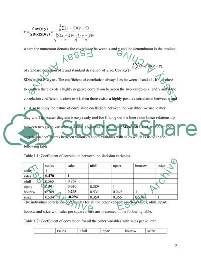
STAT Report Fashion stores will be designed and arranged in an enticing manner, so they can showcase their dresses in an elevating way thereby impressing the entering customers. “The physical construction of the buildings, the locations, and style of the stores - all these things are social constructions, but entrenched to various degrees” (Aspers 2010, p.68). Apart from the physical attributes, fashion stores need to have efficient and customer-friendly employees who can make the customers comfortable and importantly facilitate them to make that buying decision. “They have direct contact with their customers, are not bound by corporate rules, and therefore can be flexible and respond quickly to customer needs” (Stephens 2002, p. 320). So, this report focuses on the data which pertains to the study of direct annual sales of 400 Dutch fashion stores in 1990, even while discussing about the physical space and working of the employees. Pair-wise correlation coefficients Actually, any data mainly will be comprised of two types. One is nominal and other is ordinal on broad sense (Ekstrom and Sørensen 2015). Here the variables used are of second type. The variable under our study are as follows: tsales which denotes Total Sales, sales which denotes Sales per square metre, nfull which denotes Number of full timers, npart which denotes Number of part timers), hoursw which denotes Total number of hours worked and ssize which denotes Sales floor space of the store in square metres. Here in our data, all the variables are of ordinal type and we will be finding the correlation between all these variable using the formula for Karl Pearson coefficient of correlation given by the following formula: where the numerator denotes the covariance between x and y and the denominator is the product of standard deviation of x and standard deviation of y. ie. Cov(x,y)=, SD(x)= and SD(y)= . The coefficient of correlation always lies between -1 and +1. If it is close to -1, then there exists a highly negative correlation between the two variables x and y and if the correlation coefficient is close to +1, then there exists a highly positive correlation between x and y. Also to study the nature of correlation coefficient between the variables, we use scatter diagram. The scatter diagram is easy ready tool for finding out the liner / non linear relationship between two given variables at a time. (Agarwal 2010). Using Microsoft Excel, we obtain the correlation coefficients between various random variables with sales which is listed in the following table. Table 1.1: Coefficient of correlation between the decision variables   tsales sales nfull npart hoursw ssize tsales 1 sales 0.470 1 nfull 0.565 0.237 1 npart 0.391 0.050 0.289 1 hoursw 0.709 0.263 0.531 0.249 1 ssize 0.534 -0.294 0.350 0.366 0.576 1 The individual correlation coefficients for all the other variables such as tsales, nfull, npart, hoursw and ssize with sales per square metre are presented in the following table. Table 1.2: Coefficient of correlation for all the other variables with sales per sq. mtr.   tsales nfull npart hoursw ssize Sales 0.47 0.237 0.05 0.236 -0.294 Summary: The coefficient of correlation of sales with tsales is 0.47 The coefficient of correlation of nfull with sales is 0.237 The coefficient of correlation of npart with sales is 0.05 The coefficient of correlation of hoursw with sales is 0.263 The coefficient of correlation of ssize with sales is -0.294. The significance of the Karl Pearson coefficient of correlation is written by the following formula: t = =  which follows Student’s t distribution with n-2 degrees of freedom, where SE denotes Standard Error. Under Null Hypothesis Ho: The correlation coefficient is 0 ie. =0. The Standard Error of the correlation coefficient is given by the formula, . The coefficient of correlation of tsales with sales is the highest which is 0.47. It is highly significant also with probability 0.000 ( < 0.01). Therefore, it is depicted that there is a significant correlation existing between total sales and sales per square metre. The coefficient of correlation of nfull with sales is 0.237 and is highly significant with probability 0.000 ( < 0.01). Therefore, there exists a positive correlation between sales per square metre and no. of full timers. The coefficient of correlation of npart with sales is 0.05 and the probability of significance is 0.159. Therefore, there exists a positive correlation of sales with no. of part timers and it is not significant, since the probability is 0.159 ( > 0.05). The coefficient of correlation of hoursw with sales is 0.263 and the probability of significance is 0.000. Therefore, there exists a positive correlation among sales and total hours worked. The coefficient of correlation of sales floor space of the store with sales is -0.294 and probability of significance is 0.000. Therefore, there exists a negative correlation among sales and sales floor space of the store. All the scatter diagrams depicting the coefficient of correlation between sales per sq. mtr and the other variables are given through Figures 1.1 to 1.5. Figure 1.1: Graph depicting the coefficient of correlation of total sales with sales per sq. mtr The above scatter plot given in chart 1.1 depicts that the coefficient of correlation of tsales with sales is positive which depicts that there exists a positive relationship among sales per sq. mtr and the total sales. Chart 1.2: Graph depicting the coefficient of correlation of nfull with sales per sq. mtr. The above scatter plot given in chart 1.2 depicts that the coefficient of correlation of nfull with sales per sq. mtr. is positive which depicts that there exists a positive relationship among sales per sq. mtr. and the nfull. Graph 1.3: Chart showing the correlation between npart and sales per sq. mtr. The above scatter plot given in chart 1.3 depicts that the coefficient of correlation of npart with sales per sq. mtr. is positive which depicts that there exists a positive relationship among sales per sq. mtr. and the npart. Chart 1.4: Chart showing the correlation between hoursw and sales per sq. mtr. The above scatter plot given in chart 1.4 depicts that the coefficient of correlation of hoursw with sales per sq. mtr. is positive which depicts that there exists a positive relationship among sales per sq. mtr. and the hoursw. Chart 1.5: Chart showing the correlation between ssize and sales per sq. mtr. The above scatter plot given in chart 1.5 depicts that the coefficient of correlation of ssize (floor space of the store) with sales per sq. mtr. is negative which depicts that there exists a negative relationship among sales per sq. mtr. and the ssize (sales floor space of the store). Equation representing a linear regression model The equation depicting the sales per square metre on hours worked on the sales floor space of the store is given by the regression analysis given in the following table which was done in Microsoft Excel. Table 2.1: Table depicting summary output of the Regression analysis Multiple R 0.605 R Square 0.365 Adjusted R Square 0.363 Standard Error 2985.37 Observations 400 Table 2.2: Table depicting ANOVA of the regression analysis Source of variation df Sum of Squares Mean Sum of Squares F ratio Significance F Regression 2 2040854395 1020427198 114.49 0.000 Residual 397 3538239209 8912441.334 Total 399 5579093605 Table 2.3: Table depicting the regression coefficients and their significance Variables  Coefficients Standard Error t Stat P-value Lower 95% Upper 95% Intercept 5133.59 321.69 15.96 0.000 4501.15 5766.03 hoursw 37.5284 2.84 13.23 0.000 31.95 43.11 ssize -22.14 1.63 -13.63 0.000 -25.34 -18.95 From the table 2.3 depicting the regression coefficients of sales per sq. mtr on hoursw (hours worked) and ssize (sales floor space of the store), we are able to detect that the constant given by the intercept is highly influential and significant with probability 0.000 which shows that the sales per sq. mtr does not exclusively depends on the variables hoursw and ssize but also the constant 5133.59. The regression coefficients of the independent variables predicting the sales per sq. mtr are 37.5284 and -22.14 and they are highly significant. The standard error of the independent variable hoursw is 2.84 and the standard error of the independent variable ssize is 1.63 whereas the dependent variable is sales per sq. mtr. (y).The regression equation is y = 5133.59 + 37.53 * hoursw - 22.14 * ssize ----(1) (please see the Excel file attached) The above said regression equation given by the equation (1) is highly robust because the multiple correlation coefficient R is 0.6 and the coefficient of determination R2 is 0.366. Approximately 36.6% of the dependent variable, that is, sales per sq. mtr is predictable through the independent variables hoursw and ssize. The data has 400 values which are very large; therefore the regression equation seems to be more robust and precise in estimating the dependent variable sales per sq. mtr based on the two independent variables hoursw and ssize and the constant / intercept. Economic perspective and Statistical significance The regression coefficient of the dependent variable (sales per sq. mtr.) on the independent variable hoursw (hours worked) 37.53 is clearly depicting a upward influence of sales on hoursw and a downward influence of sales on ssize (sales floor space of the store.). The constant of 5133.59 is also highly influential. This is due to the fact that if the sales floor space is less, the movement of the staff will be very quick and immediate deliverance to the customers is possible. Therefore the sales may likely to go up when the sales floor space is less and also the positive influence of hoursw on the sales per sq. mtr is clearly an indication that if the hours worked by the employees is more, then the sales is likely to climb up. Sales may go up when the hours worked is more; since customers may come at any time and would expect that the sales staff should be available during their visit (Wrice 2004). This would positively influence the customers’ attitude towards the store and the sales will go up naturally. So both the independent variables hoursw and ssize are having highly influential and important in deciding the sales per sq. mtr. Full timers and part timers Table 4.1: Table depicting the summary output of regression analysis Multiple R 0.634 R Square 0.402 Adjusted R Square 0.396 Standard Error 2905.82 Observations 400 Table 4.2: Table depicting the Analysis of Variance of the regression equation Source of variation df Sum of Squares Mean Sum of Squares F ratio Significance F Regression 4 2243801304 560950326.1 66.43 0.000 Residual 395 3335292300 8443777.98 Total 399 5579093605 Table 4.3: Table depicting the regression coefficients of the regression equation Variables Coefficients Standard Error t Stat P-value Lower 95% Upper 95% intercept 3751.31 427.7 8.77 0.000 2910.46 4592.16 hoursw 32.76 3.06 10.70 0.000 26.75 38.78 ssize -23.91 1.65 -14.50 0.000 -27.15 -20.67 nfull 557.31 172.25 3.24 0.00131 218.67 895.94 npart 685 225.44 3.04 0.0025 241.78 1128.22 From the table 4.3 depicting the regression coefficients of sales per sq. mtr on hoursw (hours worked), ssize (sales floor space of the store), nfull (no. of full timers) and npart (no. of part timers), we are able to detect that the constant given by the intercept is highly influential and significant with probability 0.000 ( < 0.01) which shows that the sales per sq. mtr does not exclusively depends on the variables hoursw (hours worked), ssize (sales floor space of the store), nfull (no. of full timers) and npart (no. of part timers) but also the intercept 3751.31. The regression coefficients of the independent variables predicting the sales per sq. mtr are 32.76 (hoursw). -23.91 (hoursw). nfull (557.31) and npart (685) and they are highly significant (< 0.01). The dependent variable is sales per sq. mtr. (y).The regression equation is given by y = 3751.31 + 32.76 * hoursw – 23.91 * ssize + 557.31 * nfull + 685 * npart----(2) (please see the Microsoft Excel file attached) The above said regression equation given by the equation (2) is highly robust because the multiple correlation coefficient R is 0.634 (note that there is an improvement in the multiple correlation when the two new independent variables nfull and npart are included) and the coefficient of determination R2 is 0.402. Approximately 40% of the dependent variable ie. sales per sq. mtr is predictable through the independent variables hoursw (hours worked), ssize (sales floor space of the store), nfull (no. of full timers) and npart (no. of part timers). The 400 data values are a very large sample size and hence the regression equation seems to be more strong and precise in estimating the dependent variable sales per sq. mtr, based on the four independent variables hoursw (hours worked), ssize (sales floor space of the store), nfull (no. of full timers) and npart (no. of part timers) and the constant / intercept. So there is an improvement when the two new independent variables nfull and npart are included in the regression analysis in predicting and estimating sale (sales per sq. mtr.). Conclusion and Summary: The dependent variable sale per sq. mtr at the outset is having a strong relationship with all the independent variables except npart (individually). But when the regression equation is computed, for the first instance all the independent variables hoursw and ssize were highly influential and in the second instance all the independent variables hoursw, ssize, nfull and part were highly influential which indicates that none of the variables can be ignored in deciding the sales per sq. mtr. Not only that the intercept (constant of the regression equation) is also significant in deciding the sales per sq. mtr. So the choice of independent variables in the regression equation is highly appreciable and helps one to decide about the sales per sq. mtr. References Agarwal, BM., 2010. Business Mathematics & Statistics. Ane Books Pvt Ltd. Aspers, P., 2010. Orderly Fashion: A Sociology of Markets. Princeton University Press. Ekstrom, CT and Sørensen, H., 2015. Introduction to Statistical Data Analysis for the Life Sciences. CRC Press. Stephens, FG., 2002. Fashion: From Concept to Consumer. Pearson Education. Wrice, M., 2004. First Steps in Retail Management. Macmillan Education. Read More