Quantitative Methods Analysis - Case Study Example

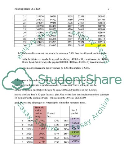
Quantitative Methods Individual 2 Week 12 Everest Brenda Jones Case Problem Tri Corporation P.756 Play the role of Tom Gifford anddevelop a simulation model for financial planning. Write a report for Tom’s boss and, at a minimum, include the following: 1. Without considering the random variability in growth rates, extend the worksheet in Figure 16.18 to 30 years. Confirm that by using the constant annual salary growth Rate and the constant annual portfolio growth rate, Tom can expect to have a 30-year Portfolio of $627,937. What would Tom’s annual investment rate have to increase to in order for his portfolio to reach a 30-year, $1,000,000 goal? a. Without considering the random variability in growth rates, extend the worksheet in Figure 16.18 to 30 years             1 14500 34000 1360 1518 17378 2 17378 35700 1428 1809 20615 3 20615 37485 1499 2136 24251 4 24251 39359 1574 2504 28329 5 28329 41327 1653 2916 32898 6 32898 43393 1736 3463 38097 7 38097 45563 1823 4582 44502 8 44502 47841 1914 4612 51028 9 51028 50233 2009 5304 58521 10 58521 52755 2110 6063 66694 11 66694 55382 2215 6891 75800 12 75800 58151 2326 7813 85939 13 85939 61059 2442 8838 97219 14 97219 64112 2564 9978 109761 15 109761 67317 2693 11245 123699 16 123699 70683 2827 12653 139179 17 139179 74217 2969 14215 156363 18 156363 77928 3117 15948 175428 19 175428 81824 3273 17870 196541 20 196541 85916 3437 19998 219976 21 219976 90211 3608 22358 245942 22 245942 94722 3789 24973 274704 23 274704 99458 3978 27868 306550 24 306550 104430 4177 31072 341799 25 341799 109652 4386 34619 380804 26 380804 115135 4605 38540 423949 27 423949 120891 4835 42878 471662 28 471662 126936 5077 47674 524413 29 524413 133283 5331 52974 582718 30 582718 139947 5598 58832 647148 b. The annual investment rate should be minimum 5.9% from the 4% mark and this is due to the fact that even standardizing and simulating 14500 for 30 years it comes to 144106. Hence the deficit to bridge the gap is (1000000-144106) = 855894 by investment only which can be increasing the investment by 1.9% thus making it 5.9%. 2. Incorporate the random variability of the annual salary growth rate and the annual portfolio growth rate into a simulation model. Assume that Tom is willing to use the annual investment rate that predicted a 30-year, $1,000,000 portfolio in part 1. Show how to simulate Tom’s 30-year financial plan. Use results from the simulation modelto comment on the uncertainty associated with Tom reaching the 30-year, $1,000,000 goal. Discuss the advantages of repeating the simulation numerous times.     Simulation with random salary Planned Inv    Sim 2 portfolio 1 14500 34000 1360 1518 17378 2 17378 34000 1428 1809 18247 3 20615 35700 1499 2136 20072 4 24251 39270 1574 2504 23082 5 28329 39270 1653 2916 24236 6 32898 41230 1736 3463 26660 7 38097 45356 1823 4582 30659 8 44502 45356 1914 4612 32191 9 51028 47624 2009 5304 35411 10 58521 52387 2110 6063 66694 11 66694 52387 2215 6891 75800 12 75800 55006 2326 7813 85939 13 85939 60507 2442 8838 97219 14 97219 60507 2564 9978 109761 15 109761 63532 2693 11245 123699 16 123699 69857 2827 12653 139179 17 139179 69857 2969 14215 156363 18 156363 73380 3117 15948 175428 19 175428 80718 3273 17870 196541 20 196541 80718 3437 19998 219976 21 219976 84753 3608 22358 245942 22 245942 93227 3789 24973 274704 23 274704 93227 3978 27868 306550 24 306550 97890 4177 31072 341799 25 341799 107679 4386 34619 380804 26 380804 107679 4605 38540 423949 27 423949 113063 4835 42878 471662 28 471662 124370 5077 47674 524413 29 524413 124370 5331 52974 582718 30 582718 130588 5598 58832 647148 Simulation Clause-1 Initial Salary Salary growth rate- 0% Salary growth rate- 5% Salary growth rate- 10% Salary growth rate- 0% Salary growth rate- 5% Salary growth rate- 10% Salary growth rate- 0% Salary growth rate- 5% Salary growth rate- 10% Salary growth rate- 0% Salary growth rate- 5% Salary growth rate- 10% Salary growth rate- 0% Salary growth rate- 5% Salary growth rate- 10% Salary growth rate- 0% Salary growth rate- 5% Salary growth rate- 10% Salary growth rate- 0% Salary growth rate- 5% Salary growth rate- 10% Salary growth rate- 0% Salary growth rate- 5% Salary growth rate- 10% Salary growth rate- 0% Salary growth rate- 5% Salary growth rate- 10% Salary growth rate- 0% Salary growth rate- 5% Simulation Clause-2 Simulation-3 Planned Portfolio original Planned Portfolio original Considering- 5% portfolio growth Considering- 15% portfolio growth Considering- 10% portfolio growth Considering- 10% portfolio growth Considering- 15% portfolio growth Considering- 5% portfolio growth Considering- 5% portfolio growth Considering- 15% portfolio growth Considering- 10% portfolio growth Considering- 10% portfolio growth Considering- 15% portfolio growth Considering- 5% portfolio growth Considering- 5% portfolio growth Considering- 15% portfolio growth Considering- 10% portfolio growth Considering- 10% portfolio growth Simulation 3 Portfolio 17378 19985 21983 23082 26544 29199 30659 35257 38784 From the above simulation1 it shows if we consider that there is a fluctuation of salary growth rate from 0% to 10% then at any level the investment planned of 4 % will be near or fall back from the investment amount required even to touch 670000$. Hence 1000000$ cannot be achieved. Coming to simulation 2 & 3 whether we take portfolio growth from 5% to 15% in ascending way or vice versa , on the third year the investment portfolio will be the same as original and hence it will be reaching 670000$ only and again 1000000$ cannot be achieved. So it is absolutely uncertain to reach 1000000$ on varying investment amount or portfolio growth and the only way to achieve is to invest 5.9% at least as projected to achieve 1000000 and only then the fluctuations can be considered to reach 1000000$. 3. What recommendations do you have for employees with a current profile similar to Tom’s after seeing the impact of the uncertainty in the annual salary growth rate and the annual portfolio growth rate? The recommendations are: 1. Invest at least 6% of your salary or even more 2. Create diverse portfolio investments 3. Should keep a vigil that there should be difference of 2% from inflation and portfolio growth rate to have the stable and projected capital after retirement. 4. Assume that Tom is willing to consider working 35 years instead of 30 years. What is your assessment of this strategy if Tom’s goal is to have a portfolio worth $1,000,000? 27 423949 120891 4835 42878 471662 28 471662 126936 5077 47674 524413 29 524413 133283 5331 52974 582718 30 582718 139947 5598 58832 647148 Considering the change of portfolio by in the successive year by an addition of 5000$ the simulation gives a figure for next 5 years Starting 30 647148   31 68000   32 73000   33 78000   34 83000   35 88000     1037148 Hence if tom works for 35 years he will reach the 1000000$ fund as projected above. 5. Discuss how the financial planning model developed for Tom Gifford can be used as a template to develop a financial plan for any of the company’s employees. The template that has been used for Tom Gifford ( simulation model with random variability) creates a realistic simulation because in the corporate industry and also considering the reaction of economic depression leading to recession salary will depend and the growth rate may be 0% and if appraisal is above satisfactory it might reach 15% with a mean of 10% and this will be the original situation for an average performer in the industry. Case Problem 2 Harbor Dunes Golf Course P.758 Develop simulation models for both replay options using Crystal Ball. Run each simulation for 5000 trials. Prepare a report that will help management of Harbor Dunes Golf Course decide which replay option to implement for the upcoming spring golf season. In prepar- ing your report, be sure to include the following: 1. Statistical summaries of the revenue expected under each replay option  25$+cart fee        50$+cart fee         Probable profit       Probable profit 0 0.01 0   0 0.06 0 1 0.03 540   1 0.09 2520 2 0.05 1800   2 0.12 6720 3 0.05 2700   3 0.17 14280 4 0.11 7920   4 0.2 22400 5 0.15 13500   5 0.13 18200 6 0.17 18360   6 0.11 18480 7 0.15 18900   7 0.7 13720 8 0.13 18720   8 0.5 11200 9 0.9 14580         10 0.6 10800         Total   107820       107520 2. Your recommendation as to the best replay option As seen from the above simulation the best replay option is the first one with 25$ + cart fee 3. Assuming a 90-day spring golf season, an estimate of the added revenue using your Recommendation The added revenue will be 300*30=9000$ 4. Any other recommendations you have that might improve the income for Harbor Dunes Recommendations will be to let the golfers to use the premium field before and after the premium time at 50$ + cart fee as it can be seen the number of less foursomes in this category has more profitability and as there is time restraint in the premium time hence this option is the most feasible one. Case Problem 3 County Beverage Drive-Thru P.760 Prepare a report that discusses the general development of the spreadsheet simulation model, and make any recommendations that you have regarding the best store design and staffing plan for County Beverage. One additional consideration is that the design allowing for a two-server system will cost an additional $10,000 to build. 1. List the information the spreadsheet simulation model should generate so that a decision can be made on the store design and the desired number of clerks. New One     Previous system   1 0.2       2 0.3   2 0.24 3 0.35   3 0.2 4 0.1   4 0.15 5 0.05   5 0.1   0.8     0.69 Total probabilitiy of served within 5 minutes =0.8(new system) Total probability of served within 5 minutes =0.69 old system) New One     Previous system   Customer % more served     1 0.2             2 0.3   2 0.24 25     3 0.35   3 0.2 75     4 0.1   4 0.15 -10     5 0.05   5 0.1 -50       0.8     0.69       Not only the probability of serving more clients is better in new system than old system in 5 minutes but even when simulated on minute on minute basis from 2 to 5 mins it is clear that with a two server system within 3 minutes 100% more customers are served than the previous system thus the profitability will also double by 2 times from present level and hence investment of $10000 seems worthy. That means the 6 minutes waiting is reduced to 3 minutes in the new system and hence 100% more servings. 2. Run the simulation for 1000 customers for each alternative considered. You may want to consider making more than one run with each alternative. [Note: Values from an exponential probability distribution with mean can be generated in Excel using the following function: *LN(RAND()).] Even after running the simulation for 1000 customers with mean fluctuations New One   total customers served Previous system   Customer % more served     1 0.2 40       0   2 0.3 120 2 0.24 25 96   3 0.35 210 3 0.2 75 120   4 0.1 80 4 0.15 -10 120   5 0.05 50 5 0.1 -50 100     0.8 500   0.69       Mean 100 clients 87.2 It seems that the mean would be always higher by 12.8 clients in new 2 server system than the old one. 3. Be sure to note the number of customers County Beverage is likely to lose due to long customer waiting times with each design alternative. References Anderson, David R., Sweeney, Dennis J., Williams, Thomas A., Camm, Jeffrey D., Cochran, James J., Fry, Michael J., Ohlmann, Jeffrey W., (2013), Quantitative Methods, 12th ed. Read More