Relationship between Depression and Demographic Variable - Assignment Example

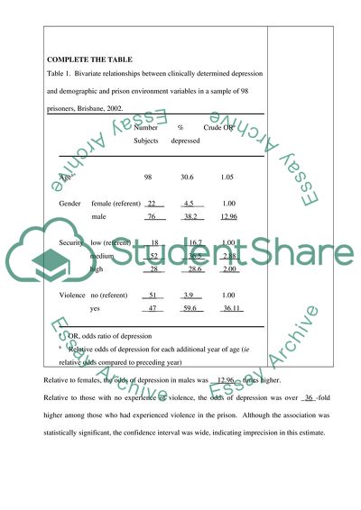
6002HLS Quantitative Research Assignment 2 number: of Convenors: Due Week 14: Friday, 11th of June, before 5pmAssignment 2: 6002HLS Quantitative Research Part I Questions (Fill in the blanks) Of the total of __98__ prisoners in this study, _22.4__ % (22) were female. Mean age of the sample was _36.41__ (SD = 7.56). About half (53.1% (52)) of the prisoners were in medium-level security, about a quarter (28.6% (28)) in high-level security, and just under a fifth (18.4% (18)) in low-level security. _48.0_ (%) (47) were victims of violence within the prison. Overall, _30_ (30.6 %) of the 98 subjects were determined to be clinically depressed. At the bivariate level of analysis, the prevalence of depression was significantly higher for males (38.2_ %) than females (4.5_ %) (Fisher’s exact test, p = 0.002). The prevalence of depression was lower (16.7_ %) in those detained in low-security environments compared to medium with the highest prevalence of depression (36.5_ %), or high security (28.6_ %) environments. However, this difference did not attain statistical significance (Likelihood ratio 22 = 2.7, p = 0.255). Prevalence of depression was significantly __higher__ for prisoners who had experienced violence during their detention. _3.9__percent of those not experiencing violence were determined to be clinically depressed compared with __59.6_% of prisoners who had experienced violence (Fisher’s exact test, p < 0.001). COMPLETE THE TABLE Table 1. Bivariate relationships between clinically determined depression and demographic and prison environment variables in a sample of 98 prisoners, Brisbane, 2002. Number % Crude ORa Subjects depressed Ageb 98 30.6 1.05 Gender female (referent) _22 _4.5___ 1.00 male _76_ _ _38.2__ 12.96 Security low (referent) __18__ __16.7_ 1.00 medium _ 52__ __36.5_ _2.88_ high _ 28 _ __28.6_ _2.00_ Violence no (referent) _ 51__ _3.9__ 1.00 yes __47__ _59.6__ _36.11_ a OR, odds ratio of depression b Relative odds of depression for each additional year of age (ie relative odds compared to preceding year) Notes ……. 1. Initially, describing the sample itself. Sets scene. 2. Concentrates on research question and hence outcome of depression. 3. Overall number depressed gives some idea of power. 4. Bivariate look at what influences depression. 5. Assumes no mutual confounding of variables involved, or by any other variables. For your calculations! Relative to females, the odds of depression in males was __12.96__ times higher. Relative to those with no experience of violence, the odds of depression was over _36_-fold higher among those who had experienced violence in the prison. Although the association was statistically significant, the confidence interval was wide, indicating imprecision in this estimate. Relationship between depression and demographic variable Relationship between Depression and Age Group There was non-significant relationship between depression and age group, χ2(2, N = 98) = 0.24, p = 0.886. However, prisoners ‘between 34 to 40 years’ and ‘over 40 years’ were about 1.19 and 1.30 times more likely to be depressed than the prisoners ‘below 33 years’. Relationship between Depression and Gender There was significant relationship between depression and gender, χ2(1, N = 98) = 9.08, p = 0.003. Male prisoners were about 12.96 times more likely to be depressed than the female prisoners. Relationship between Depression and Security Level There was non-significant relationship between depression and security level, χ2(2, N = 98) = 2.56, p = 0.278. However, prisoners kept in medium and high security level environments were about 2.88 and 2.00 times more likely to be depressed than the prisoners kept in low security level environment. Relationship between Depression and Violence There was significant relationship between depression and being victim of violence within the prison or not, χ2(1, N = 98) = 36.67, p < 0.001. The prisoners who were victim of violence within the prison were depressed about 36.11 times more than the prisoners who were not victim of violence within the prison. In conclusion, violence and gender have significant effect on depression. However, security level and age group have non-significant effect on depression. Assignment 2 Part II (1) Overall, is there improvement in range of movement over time? Range or movement at three times: MOVE1, MOVE2, MOVE3 are continuous variables. (Repeated Measures of ANOVA or Friedman test depending upon the statistical assumptions) Variables Independent variable: time before and after the surgery, which is nominal categorical variable Dependent variable: range of movement of hand in degrees, which is a continuous variable Data Analysis Method The data was collected from 96 patients from hospital outpatients clinics in four Brisbane hospitals measured at three different time points. Thus, an appropriate test would be Repeated Measures of ANOVA or Friedman test depending upon the statistical assumptions met or not. Statistical Assumptions for Repeated Measures of ANOVA Random Sampling Independence of observation Variables are Normally distributed (normality) Homogeneity of Variance that is equal variances across the group Homogeneity of Co-Variance Assumption Check Table 1 shows the summary statistics for range of movement of hand in degrees at three times. Table 1: Descriptive Statistics (N = 96) Mean SD Median Min Max Skewness Kurtosis Move 1 44.33 16.14 46 15 87 0.409 -0.097 Move 2 75.75 16.51 73 44 121 0.369 -0.153 Move 3 122.78 16.52 118 103 184 1.651 3.263 Figure 1 to 3 show the distribution of range of movement of hand in degrees at three times: Move 1 (Prior to Surgery), Move 2 (1-Month Post Surgery) and Move 3 (12-Month Post Surgery). Figure 1: Histogram of range of movement prior to surgery Figure 2: Histogram of range of movement at one month post-surgery Figure 3: Histogram of range of movement at 12-month post-surgery Mauchlys Test of Sphericity Mauchly’s test of Sphericity is used for checking the homogeneity of variance assumption for repeated measures ANOVA. The closer the Greenhouse-Geisser epsilon is to 1, the more homogeneous are the variances of differences, and thus the closer the data are to being spherical. Table 2 shows the Greenhouse-Geisser adjusted p value (0.172 ) that is greater than 0.05, indicating that there are no significant differences among 3 times in terms of variation. Thus, assumption of homogeneity of variance is met. Table 2: Mauchlys Test of Sphericity Within Subjects Effect Mauchlys W Approx. Chi-Square df Sig. Epsilon Greenhouse-Geisser Huynh-Feldt Lower-bound Time .963 3.523 2 .172 .965 .984 .500 Summary of Assumptions Table 3 summarizes the assumption for the Repeated Measures of ANOVA. As shown in table 3, normal assumption for Move 3 is violated. Thus, an appropriate test would be Friedman test. Table 3: Summary of assumptions for the Repeated Measures of ANOVA Mean 10% of Median Min (-3SD of Mean), Max(+3SD of Mean) Skewness ≤ |3| Kurtosis ≤ |3| Histogram Shape Homogeneity of Variance Move 1 √ √ , √ √ √ √ √ Move 2 √ √ , √ √ √ √ Move 3 √ √, Χ √ Χ Χ (Assumption met = √, Assumption not met = Χ) Friedman Test Table 4 shows the results of Friedman test. There are significant differences in the range of movement of hand over time, χ2(2, N = 96) = 178.26, p < 0.001. Table 4: Friedman Test Mean Rank N df χ2 sig Move 1 (baseline) 1.08 96 2 178.26 < 0.001 Move 2 1.92 Move 3 3.00 Three Wilcoxon signed-ranks test were performed (pot-hoc comparisons) to find where differences really exist, as normality assumptions for parametric test were not met. Table 5: Wilcoxon Signed-Ranks Test Median (Min, Max) Z Sig. Move1 ~ Move 2 51(15, 87) ~ 87(44, 121) -8.04 < 0.001 Move1 ~ Move 3 51(15, 87) ~ 128(103, 184) -8.51 < 0.001 Move2 ~ Move 3 87(44, 121) ~ 128(103, 184) -8.51 < 0.001 Table 5 shows the results of three Wilcoxon signed-ranks test. As shown in table 5, there are significant differences in all the three groups (p 0.05). Nagelkerke R2 of 0.216 suggests that the gender and dominant side explain about 21.6% variation in patient’s severity of the injury. Discussion The study was conducted on 96 patients with average age 23.2 years (SD = 4.3 years). Majority (52.1%) of the patients were female. Four percent females were severely injured compared to about 30.4% males, thus, severity of the injury is more in males than females. However, both non-dominant (17.4%) and dominant (16%) sides has approximately same severity of the injury. Relative to females, the odds of severity of the injury in males was 10.6 times higher. However, relative to dominant side, the odd of severity of the injury was 1.1 times higher on non-dominant side. Overall Discussion In conclusion, surgery is an effective treatment for sports-related injury, has a very good impact on range of arm movement over time and range of arm movement improves as the time passes after surgery. Patient’s range of arm movement prior to surgery does not depending on patients’ age. At baseline, severity of the injury depends on gender; however, there is no effect of dominant side on severity of the injury. Assignment 2 Part III Research Questions: 1. Is premature born infants group different from the full-term infants group in mother’s education, income, marital status and depression level? Hypotheses Hypothesis 1 H0: Term of infant birth is independent off mother’s education. H1: Term of infant birth is dependent on mother’s education. Hypothesis 2 H0: Term of infant birth is independent off mother’s annual family income. H1: Term of infant birth is dependent on mother’s annual family income. Hypothesis 3 H0: Term of infant birth is independent off mother’s marital status. H1: Term of infant birth is dependent on mother’s marital status. Hypothesis 4 H0: Term of infant birth is independent off mother’s depression level. H1: Term of infant birth is dependent on mother’s depression level. Variables Independent Variables: mother’s education and family income that are ordinal categorical variables and marital status, and depression level that are dichotomous categorical variables Dependent variable: term of infant birth, which is dichotomous categorical variable Statistical Test The selected test is non-parametric Chi-square Test of Independence, as both independent and dependent variables are categorical variables. Level of Significance The selected level of significance is 0.05. . Thus, null hypothesis will be rejected, if p-value ≤ 0.05. Statistical Assumptions for Chi-Square Test of Independence All expected frequencies are 1 or greater. At most 20% of the expected frequencies are less than 5. Results Table 1 shows the results of term of infant birth by demographic variables. Table 1: Term of infant birth by demographic variables Term of Infant Birth Pre-Term N (%) Full-Term N (%) OR χ2 (df) Sig. Mother’s Education < 10 10 (13.5) 6 (8.1) 4.03 10.73 (3) 0.013 10 to 12 38 (51.4) 25 (33.8) 3.67 Tafe and Diploma 14 (18.9) 14 (18.9) 2.42 Tertiary (referent) 12 (16.2) 29 (39.2) 1.00 Annual Family Income < 30 K 35 (47.3) 8 (10.8) 20.42 38.97 (2) < 0.001 30 to 49.9 K 30 (40.5) 24 (32.4) 5.83 50 to 79.9 K (referent) 9 (12.2) 42 (56.8) 1.00 Mother’s Marital Status Married or defecto 60 (81.1) 56 (75.7) 1.38 0.64 (1) 0.424 Single (referent) 14 (18.9) 18 (24.3) 1.00 Mother’s Depression Level Depressed 53 (71.6) 8 (10.8) 20.82 56.47 (1) < 0.001 Not Depressed (referent) 21 (28.4) 66 (89.2) 1.00 Relationship between Term of Infant Birth and Mother’s Education The percentage of infant that were born pre-term differed by mother’s education, χ2(3, N = 148) = 10.73, p = 0.013. Infants with mother’s education ‘less than 10 years’, ‘10 to 12 years’ and ‘Tafe and Diploma’ were about 4.03, 3.67 and 2.42 times more likely to be born pre-term than the infant born with mother’s education of ‘Tertiary’. Relationship between Term of Infant Birth and Mother’s Annual Family Income The percentage of infant that were born pre-term differed by mother’s annual family income, χ2(2, N = 148) = 38.97, p < 0.001. Infants with mother’s annual family income ‘less than $30,000’ and ‘$30,000 to $49,999’ were about 20.42 and 5.83 times more likely to be born pre-term than the infant born with mother’s annual family income ‘between $50,000 to $79,999’. Relationship between Term of Infant Birth and Mother’s Marital Status The percentage of infant that were born pre-term did not differed by mother’s marital status, χ2(1, N = 148) = 0.64, p = 0.424. However, infants with married or defecto mother were about 1.38 times more likely to be born pre-term than the infant born with single mother. Association between term of infant birth and mother’s depression level The percentage of infant that were born pre-term differed by mother’s depression level, χ2(1, N = 148) = 56.47, p < 0.001. Infants with depressed mother are about 20.82 times more likely to be born pre-term than the infant born with not depressed mother. In conclusion, premature born infants group is different from the full-term infants group in mother’s education, income, and depression level. However, premature born infants group is not different from the full-term infants group in mother’s marital status. 2. Are there any differences between premature born children and full-term infants in motor and mental scores? Hypotheses Hypothesis 1 H0: There is no difference between premature born children and full-term infants in motor scores. H1: There is a difference between premature born children and full-term infants in motor scores. Hypothesis 2 H0: There is no difference between premature born children and full-term infants in mental scores. H1: There is a difference between premature born children and full-term infants in mental scores. Variables Independent Variable: term of infant birth, which is dichotomous categorical variable Dependent Variables: motor and mental scores, which are both continuous variable Statistical Test The independent variable is categorical and the dependent variables are continuous, thus, an appropriate test would be Independent-samples t-Test or Mann-Whitney U-Test depending upon the statistical assumptions to be met. Level of Significance The selected level of significance is 0.05. Thus, null hypothesis will be rejected, if p-value ≤ 0.05. Statistical Assumptions for the Independent-Sample t-test Independence of observation Normally distributed continuous dependent variable Equal homogeneity of variance for Independent Variables Normality Check Table 2: Descriptive statistics (N = 148) Mean SD Median Min Max Skewness Kurtosis Mental score 102.53 12.14 104.5 78 123 -0.200 -1.043 Motor score 96.91 10.87 95 76 126 0.481 -0.356 Figure 1: Histogram of motor score Figure 2: Histogram of mental IQ score Homogeneity of Variance Table 3: Levene’s test for equality of variance N F Sig. Mental score 148 9.053 0.003 Motor score 148 0.002 0.962 Summary of Assumptions Table 4 summarizes the assumption for the Independent-Sample t-test. As shown in table 4, all the assumptions for motor score is satisfied, however, for mental score assumption of homogeneity of variance is violated. Therefore, a Mann-Whitney U test will be performed for mental score and an Independent Samples t-Test will be performed for motor score. Table 4: Summary of assumptions for the Independent-Sample t-test Mean 10% of median Min (-3SD of mean), Max(+3SD of mean) Skewness ≤ |3| Kurtosis ≤ |3| Shape of histogram Homogeneity of variance Mental Score √ √ , √ √ √ √ Χ Motor Score √ √, √ √ √ √ √ (Assumption met = √, Assumption not met = Χ) Results Table 5 and 6 shows the results of Independent-samples t-Test for motor scores and Mann-Whitney U-Test for Mental scores. Table 5: Independent Samples t-Test for motor score Term of Infant Birth 95% CI for Mean Difference   Pre-Term Post-Term   Mean (SD) Mean (SD) df t p-value Motor Score 93.80 (10.86) 100.01 (10.02) 146 -3.619 < 0.001 (-9.611, -2.822) Table 6: Mann-Whitney U test for mental score Term of Infant Birth   Pre-Term Post-Term   Median (Min, Max) Median (Min, Max) Z p-value Mental Score 91 (78, 115) 111 (98, 123) -8.964 < 0.001 An Independent Samples t-Test indicated that there is a significant difference between premature born children and full-term infants in motor scores, t(146) = -3.62, p < 0.001. Pre-term born infants (M = 93.80, SD = 10.86) reported lower motor score of development quotient than post-term born infants (M = 100.01, SD = 10.02). A non-parametric Mann-Whitney U test indicated that there is a significant difference between premature born children and full-term infants in mental scores, z = 8.96, p Read More