Logistics and Transportation Planning - Assignment Example

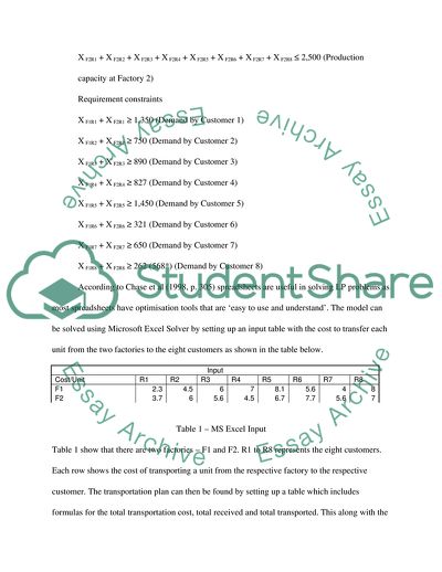
Logistics and Transportation Planning Part A According to Reed and Leavengood (2002) solving transportation problems represents one of the most successful applications of quantitative analysis. The mathematical model that minimizes the transportation cost at TNLogistics Company is the linear programming (LP) transportation model (Heizer and Render 2011). This model requires three different sets of numerical values. They are the capacity of the plant, customer demand, and the transportation cost per unit from each factory to each customer. In this case there are two factories with a total capacity of 6,500 per months and eight customers with forecasted demand totalling 6,816. This makes the demand greater than the capacity of the factory for a given month. The transportation model is structured in the following way: Objective – Minimise transportation cost subject to the following constraints. Constraint #1 – Total number of products sent from the two factories is ≤ factory capacity Constraint #2 – Total number of products demanded ≥ customer demand. The mathematical model that would minimise transportation cost at TNLogistics is: Minimise: $2.3XF1R1 + $4.5XF1R2 + $6XF1R3 + $7XF1R4 + $8.1XF1R5 + $5.6XF1R6 + $4XF1R7 + $8XF1R8 + $3.7XF2R1 + $6XF2R2 + $5.6XF2R3 + $4.5XF2R4 + $6.7XF2R5 + $7.7XF2R6 + $5.6XF2R7 + $7XF2R8 Subject to the following: Capacity constraints X F1R1 + X F1R2 + X F1R3 + X F1R4 + X F1R5 + X F1R6 + X F1R7 + X F1R8 ≤ 4,000 (Production capacity at Factory 1 X F2R1 + X F2R2 + X F2R3 + X F2R4 + X F2R5 + X F2R6 + X F2R7 + X F2R8 ≤ 2,500 (Production capacity at Factory 2) Requirement constraints X F1R1 + X F2R1 ≥ 1,350 (Demand by Customer 1) X F1R2 + X F2R2 ≥ 750 (Demand by Customer 2) X F1R3 + X F2R3 ≥ 890 (Demand by Customer 3) X F1R4 + X F2R4 ≥ 827 (Demand by Customer 4) X F1R5 + X F2R5 ≥ 1,450 (Demand by Customer 5) X F1R6 + X F2R6 ≥ 321 (Demand by Customer 6) X F1R7 + X F2R7 ≥ 650 (Demand by Customer 7) X F1R8 + X F2R8 ≥ 262 (568*) (Demand by Customer 8) According to Chase et al (1998, p. 305) spreadsheets are useful in solving LP problems as most spreadsheets have optimisation tools that are ‘easy to use and understand’. The model can be solved using Microsoft Excel Solver by setting up an input table with the cost to transfer each unit from the two factories to the eight customers as shown in the table below. Input Cost/Unit R1 R2 R3 R4 R5 R6 R7 R8 F1 2.3 4.5 6 7 8.1 5.6 4 8 F2 3.7 6 5.6 4.5 6.7 7.7 5.6 7 Table 1 – MS Excel Input Table 1 show that there are two factories – F1 and F2. R1 to R8 represents the eight customers. Each row shows the cost of transporting a unit from the respective factory to the respective customer. The transportation plan can then be found by setting up a table which includes formulas for the total transportation cost, total received and total transported. This along with the constraints indicated above will be input to the section on the spreadsheet where the results will be located. In order to solve the transportation problem the solver should be selected from the analysis section of the Microsoft Excel tool bar. A dialog box entitled ‘solver parameters’ will appear. The dialog box requires the identification of the target cell (the objective function – which is to minimise the total transportation cost), the changing cells (decision variables – the cells that will contain the number of units of the product to be supplied to each of the eight customers from each of the two factories), and the constraints (factory capacity and number of products demanded by each customer) (Chase et al 1998). The ‘Target Cell’ contains the formula for the total transportation cost. The ‘Changing Cells’ contain the results which Solver will provide so that the value in the ‘Target Cell’ can be calculated. The box which requires information on ‘Subject to the Constraints’ helps to ensure that the results are less than or equal to the factory capacity in the case of the capacity constraint, and greater than or equal to in the case of the demand constraints. After the information has been provided the final step is to choose the option which requires the Solver to ‘Solve’ the problem. The Microsoft Excel Solver output would be as follows. Microsoft Excel Solution Transport plan R1 R2 R3 R4 R5 R6 R7 R8 Total Transported   Plant Capacity F1 546 538 502 515 946 273 438 244 4,000 = >= >= >= >= >= >=       Total demand 1,350 750 890 827 1,450 321 650 262                               Total Transportation cost 36,073.10                     Table 2 – MS Excel Solution Table 2 shows the generated solution for MS Excel Solver. The total transportation cost arrived at in this model is $36,073.10. Although, at least 568 units are demanded by Customer 8 (R8), only 262 can be provided. This was done in order to enable the amount demanded to equate with the capacity of the two factories at TNLogistics capacity so that a feasible solution could be obtained. The quantity for customer 8 was reduced because the transport cost per unit to get the goods to the location is relatively higher than all the other customers. The solution provided by MS Solver can be improved. The following table provides an improvement using the Intuitive Lower-Cost Method. Intuitive Lowest-Cost Method Transport plan R1 R2 R3 R4 R5 R6 R7 R8 Total Transported   Plant Capacity F1 1,350 750 890 0 0 321 650 39 4,000 = >= >= >= >= >=       Total customer demand 1,350 750 890 827 1,450 321 650 578                               Total Transportation cost 31,527.10                     Table 3 – The intuitive lower-cost method The intuitive lowest-cost method makes initial allocations based on the lowest cost (Heizer and Render 2011). The following steps were applied in accordance with Heizer and Render (2011). Step 1 – The cell with the lowest cost is identified Step 2 – As many units as possible was allocated without exceeding the demand or supply. Step 3 – The cell with the lowest cost from the remaining cells is chosen. Step 4 – Steps 2 and 3 are repeated until all units have been allocated The factory output is less than customer demand and so a dummy factory was introduced in order to account for the excess demand. The total minimum transportation cost is $31,527.10. The limitations of the model are that lLP is static and therefore does not take into account changes over time (Simchi-Levi et al (2008). A key requirement of LP is that all the constraints along with the objective function must be linear. However, in real life problems are not linear. Only one objective can be dealt with in any one solution – profit maximisation or in this case minimisation of transport cost. In this case, the model did not provide consistent solutions when MS Solver is used. The model requires that demand equates with supply. In order to get over this the demand from customer 8 was reduced in order to arrive at a feasible solution. However, it is recommended that dummy variables be added (Factory 3 in this case) to account for the shortfall in capacity. Part B There are a number of techniques that are used to solve location problems. The centre of gravity method is useful in this regard. It also takes into account the location of the factories, location of customers, volume of goods transported and transportation cost in arriving at the best location for the distribution centre (Kumar and Suresh 2009, p.38). The aim of this method is to minimise the weighted distance between the factory and its supply and distribution points, so therefore the distance is weighted by the number of items supplied or consumed (Kumar and Suresh 2009). TNLogistics Company has a total of eight customers and two factories and so this technique provides the best means of arriving at a location for a regional distribution centre that will allow the firm to minimise the cost of transporting goods to customers. The mathematical model that minimises the total distance from the new distribution centre is as follows: Cx = (ƩDix*Wi)/∑Wi Cy = (ƩDiy*Wi)/∑Wi Cx represents the x coordinate of the centre of gravity; Cy - the y coordinate of the centre of gravity; Dix the x coordinate of location l, and Diy – the y coordinate of location l. The location of the new distribution centre that will serve the eight customers of TNLogistics can be found from the information in the following table. Retailer x, y Demand (i) Lx Ly R1 4, -3 1,350 5400 -4050 R2 6, 8 750 4500 6000 R3 21, 12 890 18690 10680 R4 34, -11 827 28118 -9097 R5 7, -2 1,450 10150 -2900 R6 -1, -21 321 -321 -6741 R7 -4, 7 650 -2600 4550 R8 -7, 15 578 -4046 8670    Total 6816 59891 7112 Table 4 – Centre of Gravity Results Table 4 provides information on the coordinates for TNLogistics Company’s customers. The demand by each customer is weighted separately with the x and y coordinates. From the information in the table the following values were calculated. Cx = ƩLx/Ʃi = 59891/6816 = 8.79 Cy = ƩLy/Ʃi = 7112/6816 = 1.04 The Centre of gravity is (8.79, 1.04) The coordinates for the centre of gravity is (8.79, 1.04) and this is the vicinity in which the distribution centre will be located in order to minimise transportation costs. Part C According to Paessens (1988) the routing of vehicles is a challenging logistics management problem as it can solve many problems including dispatch of delivery trucks. TNLogistics needs to route products from the distribution centre to retailers. The objective of any saving algorithm is to develop a set of vehicle routes which will ensure that all customers are served and that customers’ demand are met. The constraints on the problem are: only one (1) vehicle available; and the capacity of the vehicle is 1,800 units. In solving the problem the routing plan needs to take into consideration customer location in relation to the distribution centre as well as quantity demanded. The savings occur when more than one customer located in close vicinity are served on the same route, thereby merging some routes. The following input data will be used to solve the vehicle routing problem (VRP): n = 8 customers 0 = distribution centre di = (0, 1350, 750, 890, 827, 1450, 321, 650, 568) demands Distance matrix = {di,j} = ij 0 1 2 3 4 5 6 7 8 0 0 5 3 12 25 2 10 13 16 1 5 0 2 17 30 3 5 8 11 2 3 2 0 15 28 1 7 10 13 3 12 17 15 0 13 14 22 25 28 4 25 30 28 13 0 27 35 38 41 5 2 3 1 14 27 0 8 11 14 6 10 5 7 22 35 8 0 3 6 7 13 8 10 25 38 11 11 0 3 8 16 11 13 28 41 14 14 3 0 Table 5 – Euclidean Distance Matrix Q = 1800 vehicle capacity Initially, the vehicle served each customer separately. However, a merger of two or more routes can result in a reduction in transportation cost. The question is – If we merge routes i = 3 and i = 4, How much is saved? s(i, j) = d(D,i) + d(D, j) – d(i, j) If sij > 0, then the merger operation is deemed to be convenient. The vehicle is said to be overloaded if customers 1 and 2 which are not feasible mergers is carried out. The following would result: Route = d(1350) + d(750) = 2100 Q = 1800 Route > Q The route 0→1→2→0 is not feasible and therefore a merger is not possible. Clarke and Wright’s algorithm starts by establishing a route for each customer. In this case there would be eight routes and eight customers. All savings values are stored in the half matrix denoted M. The higher the value of saving, the more appealing the merger operations will be. According to web.mit.edu (n.d) Clarke and Wright 1964 savings algorithm is as follows: Step 1 – calculate the savings s(i, j) = d(D, i) + d(D, j) – d(i, j) for each pair (i, j) of customer demand point. Step 2 – rank the savings s(i, j) and list them in descending order of magnitude. Step 3 – For each saving s(i, j) that is considered, include in a route if capacity constraints are not being violated, and if: a) Either, neither i nor j have been assigned in which case a new route is started including both i and j. b) Or, exactly one of the two points has already been included in a route, Step 4 – Return to step 3 until the savings list is exhausted The results in the Table 5 represent the Euclidean distance. The Euclidean distance is the distance between two points in Euclidean space. It is the absolute value of the difference between coordinates. It is the first coordinate of the first point less the first coordinate of the second point. From this the savings objects are calculated in the Matrix M below. Matrix M   1 2 3 4 5 6 7 8   1 6 0 0 4 10 10 10   2 0 0 4 6 6 6   3 24 0 0 0 0   4 0 0 0 0   5 4 4 4   6 20 20   7 26   8                   The matrix shows the savings to be obtained at the relevant coordinate. A list is then created as shown below. List sij i j 26 7 8 24 3 4 20 6 8 20 6 7 10 1 8 10 1 7 10 1 6 6 1 2 6 2 6 6 2 7 4 1 5 4 2 5 4 5 6 4 5 7 4 5 8 The List shows the savings to be achieved if certain customers are served in the same route. Customers 7 and 8 are on the route with the greatest saving of 26 and so the route (0, 7, 8, 0) is created. This is followed by customers 3 and 4 who are is on the route (0, 3, 4, 0). The routes shaded in green do not violate the constraints but are not as efficient as those shaded in blue. The routes shaded in red violate the capacity constraints and were therefore rejected. Customers 2 and 5 will therefore have routes (0, 2, 0) and (0, 5, 0) respectively. The savings obtained from performing this algorithm is 60 and the initial routes have been reduced from eight to five. References Chase, R.B., Aquilano, N.J. and Jacobs, F.R. (1998). Production and Operations Management: Manufacturing and Services. 8th ed. USA: Irwin McGraw-Hill Heizer, J. and Render, B. (2011). Principles of Operations Management. 8th ed. USA: Prentice Hall Kumar, S.A. and Suresh, N. (2009). Operations Management. New Delhi: New Age International Publishers MIT.edu. (n.d.). Single-Depot VRP. [Online] Available at: http://web.mit.edu/urban_or_book/www/book/chapter6/6.4.12.html. [Accessed 14th Jan 2012) Paessens, H. (1988). Theory and Methodology: The savings algorithm for the vehicle routing problem: European Journal of Operational Research, 34 (1988), p. 336 --344 Reeb, J. and Leavengood, S. (2002). Transportation Problem: A Special Case for Linear Programming Problems. Operations Research. June 2002 Simchi-Levi, D., Kaminsky, P. and Simchi-Levi, E. (2008). Designing and Managing the Supply Chain: Concepts, Strategies and Case Studies. 3rd ed. USA: McGraw-Hill/Irwin Read More