Handy Hydraulics Industries - Essay Example

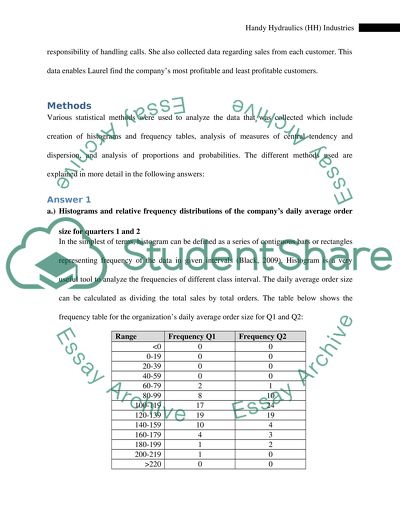
?College Handy Hydraulics (HH) Industries Business Data Analysis Statistical analysis of available data is a very important aspect of decision making for an organization. Handy Hydraulics has been collecting large amounts of data, but still decision making was primarily driven by experience and gut feelings. The objective of this report is to analyze the available data for Handy Hydraulics and find suitable strategies. Various statistical techniques such as analysis of the frequency distributions, analysis of measures of central tendency (mean, median, mode) and dispersion (variance, standard deviation, interquartile ranges), and probability analysis. The distribution of sales from each customer is analyzed to identify the most important customers. The call times for various calls are analyzed to identify the number of employees that need to be kept. Based on the analysis done, it is evident that company needs to analyze its performance with respect to quarter as well as profit center. The company needs to have 5 employees making sales calls. At the same time, the company was able to identify the most profitable customers on whom it needs to focus on. Introduction Laurel McRae has recently joined Handy Hydraulics for data analysis and strategic planning. In order to analyze the performance of the sales of the organization, Laurel collected the data for the sales for third and fourth quarter of 1990 and first and second quarter of 1991. She also collected the data regarding the machines and the days when they are working and various alternatives to replace the existing system. Number of calls received per hour was collected to analyze the sales call being made and number of employees that shall be entrusted with the responsibility of handling calls. She also collected data regarding sales from each customer. This data enables Laurel find the company’s most profitable and least profitable customers. Methods Various statistical methods were used to analyze the data that was collected which include creation of histograms and frequency tables, analysis of measures of central tendency and dispersion, and analysis of proportions and probabilities. The different methods used are explained in more detail in the following answers: Answer 1 a.) Histograms and relative frequency distributions of the company’s daily average order size for quarters 1 and 2 In the simplest of terms, histogram can be defined as a series of contiguous bars or rectangles representing frequency of the data in given intervals (Black, 2009). Histogram is a very useful tool to analyze the frequencies of different class interval. The daily average order size can be calculated as dividing the total sales by total orders. The table below shows the frequency table for the organization’s daily average order size for Q1 and Q2: Range Frequency Q1 Frequency Q2 220 0 0 Table 1: The frequency distribution table for daily average order size for Q1 and Q2 As can be seen from the table, majority of the frequency is concentrated towards the middle. The frequencies for Q1 as well as Q2 are 0 for all the intervals till the average order size of 59. While there is no daily average order size above 220 for Q1, there is no daily average order size above 200 for Q2. The best way to analyze this frequency distribution table is to analyze the histogram. The graph below shows the histogram for the company’s daily average order size for Q1 and Q2: Figure 1: Histogram of company’s daily average order size for Q1 and Q2 As can be seen from the graph, the frequency for both the seasons can be thought of following a normal curve. For Q2, the highest frequency is in the range of 100-119, while for Q1, the highest frequency is in the range of 120-139. b.) Quarterly charts for the company’s total number of orders per day The table below shows the frequency distribution for the total number of orders per day for all the four quarters: Range Frequency Q1 Frequency Q2 Frequency Q3 Frequency Q4 100-109 1 1 1 0 110-119 1 0 1 0 120-129 1 0 4 2 130-139 3 0 2 2 140-149 3 2 14 5 150-159 9 7 16 10 160-169 12 7 13 15 170-179 14 19 10 9 180-189 7 13 1 8 190-199 4 9 1 8 200-209 5 4 0 3 210-219 1 1 0 1 220-229 1 1 0 0 230-239 0 0 0 0 >240 0 0 0 1 Table 2: The frequency distribution table for total number of order for all 4 quarters The bar graph for the frequency of company’s total number of order per day for all the four quarters is shown below: Figure 2: Histogram of total number of orders per day for all 4 quarters For Q1, the highest frequency is for the range of 170-179 with 14 as the count of number of days which had 170 and 179 orders per day. For Q2, the highest frequency is 19 with 19 days having number of orders as between 170 and 179. As compared to Q1 and Q2, the frequency distribution is slightly skewed more towards the right for Q3 (Wegner, 2010). This indicates that the frequency is higher for lesser number of orders per day for Q3. The highest frequency for Q3 is 16 for the range of number of orders 150 to 159. For Q4, 15 days had number of orders between 150 and 159 which is the highest frequency for the quarter as well. This frequency distribution indicates that the total number of orders per day is higher in Q1 and Q2 as compared to Q3 and Q4. c.) Changing patterns from quarter to quarter In the case of daily average order size, the highest frequency for the average daily order size is 24 for Q2 and 19 for Q1. The average daily order size is higher for Q1 as compared to Q2. In the case of number of daily orders, the number of days having higher number of orders per day is highest for Q2 with 19 days having number of orders between 170 and 179. The daily number of orders has decreased from Q1 and Q2 to Q3. The two graphs indicate that while the average daily order size is higher for later parts of the year (Q3 and Q4) is more than that of other quarters, the number of orders per day is more for earlier quarters of the year (Q1 and Q2). Answer 2 a.) Mean, median and mode for the quarterly data on number of orders and average order size The table below shows the mean, median and mode for number of orders and average order size for the four quarters: Number of orders Average order size Q1 Q2 Q3 Q4 Q1 Q2 Q3 Q4 Mean 171.25 177.81 155.82 171.67 126.01 119.93 149.51 120.68 Median 171.5 177 156 168.5 125.74 116.71 132.98 120.09 Mode 177 191 150 163 #N/A #N/A #N/A #N/A Table 3: The measure of central tendency for number of orders and average order size for all quarters Mean, median and mode are the most common measures of central tendency that can be used to represent the entire set of data. While, mean can be calculated as the sum of all observations divided by the number of entries, median is the value that divides the distribution in two equal parts such that half of the data is less than the point, while half of the data is greater than the median. Mode is the value that is repeated most often in the data set (Bajpai, 2009). The comparison of the mean for the number of orders for 4 quarters indicates that the mean is highest for Q2 with almost 178 orders on an average per day. The median for the number of days is highest for Q2 and smallest for Q3 indicating that the distribution of number of orders is rightly skewed towards Q3. The average value of average order size is highest for Q3. The median value of the average order size for Q1, Q2, Q3 and Q4 is 125.74, 116.71, 132.98 and 120.09 respectively. From the analysis, it is evident that while the number of orders is highest for Q2, the average order size is highest for Q3. This is consistent with the findings of histogram and support Laura’s findings. The most appropriate measure of central tendency depends upon the type of data that is under study. The measurement data that is there for number of orders and average order size is ratio. The data is skewed for total number of orders per day while it is relatively symmetrical for the average order size. This implies that the most appropriate measure of central tendency for number of orders and average order size is median and mean respectively (QuickMBA, 2011). The table below shows the total sales in dollars for the last four quarters: Total Sales Dollar Q1 Q2 Q3 Q4 Sales 1,346,084.00 1,368,181.00 1,482,788.00 1,327,508.00 Table 4: Total Dollar sales for 4 quarters As can be seen from the graph, the total dollar sales is highest for Q3. It is the lowest for Q4. The total sales are doing well but can be improved. b.) Mean number of daily orders and order size for Profit Centre 3 (Pennsylvania) over the last four quarters The table below shows the mean number of daily orders and order size for profit 3: Mean no. of daily orders for profit center 3 28.17 Mean no. of daily sales for profit center 3 2780.221 Average order size for profit center 3 98.69454 Table 5: Mean number of daily orders and order size for Profit Centre 3 (Pennsylvania) As can be seen from the table, the average number of daily orders for Pennsylvania is 28, while the average order size is about 99 for the same. It can be seen that this ie considerably less than that of the entire organization. This can be partly attributed to 0 sales for profit center 3 for some part of Q3. Even after removing days having 0 as the number of orders, the average number of daily orders is 31.67 which is significantly smaller than that of profit center 2 and 1. While the average number of daily orders for profit center 2 is 45.5, the same is 95.41 for profit center 1. This indicates that there is significant difference in the average number of daily orders and the average order size for all the three profit centers. Therefore, it is necessary to analyze the performance of each profit center. Answer 3 a.) Interquartile ranges of the average order size in each quarter Interquartile range is a measurement of the dispersion of the distribution. The interquartile range can be defined as the difference between the upper and the lower quartiles (Upton and Cook, 1996). The table below shows the quartiles and the interquartile range of the average order size for the four quarters and consolidated data: Q1 Q2 Q3 Q4 Overall 1st Quartile 108.9314 107.0388 116.9412 106.3325 107.9182 3rd Quartile 142.0064 127.2414 155.882 133.1664 141.3484 Interquartile range 33.07502 20.20251 38.94072 26.83394 33.43021 Table 6: Interquartile range for the average order size for all the four quarters As can be seen from the table, the interquartile range is highest for Q3 and lowest for Q2. It is also greater than the overall interquartile range. The interquartile range for Q1 is 33.07 which is almost equal to the overall interquartile range. The interquartile range for Q2 (20.20) is significantly smaller than the overall interquartile indicating that the distribution of Q2 average order size is significantly less dispersed as compared to the overall data distribution. The interquartile range of Q4 is 26.83 which is smaller than the overall range. b.) Quarterly sample variance, standard deviation and coefficient of variation values for both the number of orders and the average order size The most common measure of variation is the standard deviation. The square of the standard deviation is called the sample variance (MIT, 2011). The coefficient of variation is a measurement of variability in relation to the mean and is used to compare the dispersion for two types of data (Jim Wright, 2011). It can be calculated as: The table below shows the parameters for all quarters for no. of orders and avg. order size: Number of orders Average order size Q1 Q2 Q3 Q4 Q1 Q2 Q3 Q4 Sample variance 548.39 336.95 281.34 467.72 702.68 597.08 582.41 582.41 Std. Dev 23.42 18.36 16.77 21.63 26.51 24.44 24.13 24.13 C.V 0.14 0.10 0.11 0.13 0.21 0.20 0.16 0.20 Table 7: Coefficient of variation, and standard deviation for number of orders and average order size for all four quarters For number of orders, the CV is highest for Q1 indicating maximum variation, while the average order size is having almost equal CV for Q1, Q2 as well as Q4. This indicates that there is less variation in the average order size. c.) Coefficient of variation for all three warehouses The table below shows the coefficient of variation for all three warehouses: Number of orders Average order size W1 W2 W3 W1 W2 W3 Std. Dev 15.84 9.97 11.89 88.01 33.29 32.25 Mean 95.42 45.59 28.17 155.85 88.29 99.01 C.V 0.17 0.22 0.42 0.56 0.38 0.33 Table 7: Coefficient of variation, and standard deviation for number of orders and average order size for three warehouses As can be seen for the number of orders, the C.V is highest for warehouse 3. This is also evident from the data where there are days with 0 number of orders. The coefficient of variation for average order size is highest for warehouse 1 indicating maximum variance. d.) Recommendations Based on the value, it is evident that while the variation in average order size does not vary across four quarters, the number of orders has significant variance across the four quarters with Q1 having the maximum CV. In order to stabilize the number of orders for all the four quarters, the company can run promotional schemes and discounts in quarters witnessing less sales. For warehouses, W3 is having the most significant variation in the number of orders, while W1 is having the highest CV for average order size. This indicates that the price is having highest variation for warehouse 1, which makes it necessary for the warehouse managers to control prices and discounts. Answer 4 a.) Probability that a machine will be down on any given day: Number of days Machine 1 is up = n1 = 223 Number of days Machine 2 is up = n2 = 223 Total number of days = n = 250 i) Probability of only one machine being down ii) Probability of both machines to be down b.) Number of days i) Number of days of only one machine being down = 0.192 * 250 = 48.168 ii) Number of days of both machine being down = 0.011 * 250 = 2.916 Answer 5 a.) Expected yearly cost of current situation Average number of days when one machine is down = n1 = 48.17 Average number of days when both machines are down = n2 = 2.916 Service call cost for one machine = s1 = 68 Service call for both machines = s2 = 100 Number of copies lost per day = c = 150 Total number of copies lost per year = N = 8100 Copier downtime cost per day = C = 0.05 Total downtime cost = N*C = 405 Total expected yearly cost = 3,972 Answer 6 Option I Total lease expense for 3 years = 12600 Probability of machine being down on a day = 0.05 Number of days in three years when 1 machine is down = 37.5 Total outgo for service calls = 0 Total no of copies lost = 11250 Total cost of copies lost = 562.5 Total cost for Option I = $13,162.50 Option II One-time investment = 8750 Per service call charge = 175 Probability of being down = 0.017 Service calls expected in 2nd and 3rd year = 8.5 Total outgo for service calls = 1487.5 "No. of days in three years when the machine will be down" = 12.75 Total no. of copies lost = 1912.5 Total cost of copies lost = 95.625 Total cost for Option II = $10,333.13 As can be seen from the analysis, Option II is less costly as compared to Option I. Answer 7 a.) The average number of calls received per hour is shown in the table below: Hour Average number of calls received per hour 8 14.50 9 26.32 10 27.91 11 31.55 12 23.77 1 30.73 2 38.86 3 34.27 4 19.50 Overall 27.49 Table 8: Average number of calls received per hour b.) Number of reps to be recommended for being 98% sure that a sales rep has to deal with only 8 calls per hour: The average number of calls per hour over all the 8 hours is 27.49. However, the highest number of calls received per hour is 38.86, while the highest number of calls received per hour is 48. In order to be 98% sure that a sales rep has to deal with only 8 calls per hour, 6 reps will be needed. c.) Stan handles only 2 calls per hour. This means that the remaining call will have to be handled by other representatives. This imply that in order to be 98% sure that the other sales rep attend only 8 calls per hour, it is needed that 6 reps will be handled the responsibility of handling calls. Answer 8 a.) Distribution of customers’ purchases The diagram below shows the distribution of customers’ purchases: Figure 3: Histogram of the frequency of the customer purchases As can be seen from the graph, the distribution is normal in nature with maximum frequency as the center and decreasing frequencies along the tail (Asad and Hailaya, 2001). b.) Mean, median and standard deviation of the distribution The table below shows the descriptive statistics of the amount spent by different customers: Mean $ 13,705.89 Median $ 13,291.50 Standard Dev $ 4,396.79 Table 9: Descriptive statistics for the amount spent by customers As can be seen from the table, the average value of the amount spent by customers is $ 13,705. The standard deviation of the distribution is $ 4,396. c.) Proportions i) Proportion of customers would be expected to have accounts greater than $20,000 From the normal table (Levin and Rubin, 2007), Proportion of accounts greater than 20,000 = 7.64% ii) Proportion of customers would be expected to have accounts less than 10,000 From the normal table, Proportion of accounts lesser than 10,000 = 20.05% iii) Actual proportions Proportion of accounts greater than 20,000 = 6.25% Proportion of accounts lesser than 10,000 = 16.25% Conclusion Analysis of HH industries indicate that the average daily order size is higher for later parts of the year (Q3 and Q4) is more than that of other quarters, the number of orders per day is more for earlier quarters of the year (Q1 and Q2). The company should look to analyze the reasons for this trend. If the higher sales are coming at the cost of discounts, company might look to find a best fit between the sales made and the order size. It is also evident that the average number of daily orders and the average order size is significantly less for Profit Center 3 as compared to other profit centers which mean that the management should look to improve the performance through promotional schemes in the region. Based on the analysis, HH should purchase the new state-of-the-art machine which would replace their old copiers. It is also important for HH to have 6 people to handle their calls in order to ensure that an individual has not to handle more than 8 calls. References Asad, Abubakar & Hailaya, Wilham. 2001. Statistics as Applied to Education and Other Related Fields. Rex Book Store Inc. Bajpai, N. 2009. Business Statistics. Pearson Education India. Black, Ken. 2009. Business Statistics: Contemporary Decision Making, 6th ed. John Wiley and Sons. Jim Wright. 2011. Measures of Dispersion: Coefficient of Variation. [Online]. Available at: http://www.jimwright.org/WebEd/u02/we020304.htm. [Last accessed on 12th May 2011]. Levin, R.I., and Rubin, D.S. (2007). Statistics for Management, 4th ed. Pearson Prentice Hall. MIT. 2011. Variance, Standard Deviation and Coefficient of Variation. [Online]. Available at: http://web.mit.edu/10.001/Web/Course_Notes/Statistics_Notes/Visualization/node4.html. [Last accessed on 12th May 2011]. QuickMBA. 2011. Central Tendency. [Online]. Available at: http://www.quickmba.com/stats/centralten/. [Last Accessed on 12th May, 2011]. Upton, Graham & Cook, I. 1996. Understanding Statistics, ill. Ed. Oxford University Press. Wegner, Trevor. 2010. Applied Business Statistics: Methods and Excel-Based Applications, 2nd ill. Ed. Juta and Company Ltd. Read More