Presenting the Categorical Data - Dissertation Example

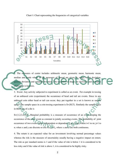
PART I: KIVZ-CHANNEL 5 TELEVISION CASE STUDY AND DATA BASE The appropriate method of presenting the categorical data is Frequency table along withbar chart or pie chart whereas the appropriate method of representing numerical data is using Descriptive Statistics and Histogram. For example with the given problem of KIVZ Channel 5 Television Case Study, the variables from X1 to X13 and X16 are categorical variables and the variables X14, X15, X17, X18 and X19 are numerical variables. The frequency table for the variables from X1 to X13 and X16 is given below Table1: Frequency table Variable Value Total 0 1 2 3 4 5 6 X1 1 13 9 21 6 0 0 50 X2 0 9 25 11 5 0 0 50 X3 0 3 5 24 12 6 0 50 X4 0 5 5 17 13 10 0 50 X5 0 7 8 14 13 8 0 50 X6 0 1 8 23 7 11 0 50 X7 0 4 5 19 11 11 0 50 X8 0 1 6 26 15 2 0 50 X9 0 14 33 3 0 0 0 50 X10 0 22 28 0 0 0 0 50 X11 0 3 1 45 1 0 0 50 X12 0 34 13 3 0 0 0 50 X13 0 8 42 0 0 0 0 50 X16 0 2 15 4 8 13 8 50 Chart 1: Chart representing the frequencies of categorical variables 2. The measures of centre includes arithmetic mean, geometric mean, harmonic mean, median and mode where as the measures of spread are given by range, mean deviation, quartile deviation and standard deviation. The measures of shape are skewness and measures of position is kurtosis. 3. Event: Any activity subjected to experiment is called as an event. For example in tossing of an unbiased coin (experiment) the occurrence of head and tail are events. Since in any unbiased coin either head or tail can occur, they put together in a set is known as sample space. The sample space in a coin tossing experiment is S={H,T}. Similarly the sample space in throwing of a die is S={1,2,3,4,5,6}. Marginal probability is a measure of occurrence of an event keeping the occurrence of the other event as constant in jointly occurring events. The probability of joint occurrence of two events either independent or dependent is p(x,y)=pij where i=1 to m; j=1 to n; when x and y are discrete or else f(x,y)=fxy where x and y are both continuous. 4. The return is an expected value for an investment involving normal percentage values whereas the risk is the measure of uncertainity usually having a negative impact on return. The risk as per standard norms is 1 and if the value of risk is below 1 it is considered to be less risky and if the value of risk is above 1, it is considered to be highly risky. Suppose the return and risk involved in an investment is given in the following table as Table 2: Sample table indicating nature of investment Investment nature Stocks Bonds Real Estate Probability for investing 0.4 0.25 0.35 Return % 13% 8% 10% Risk 1.2 0.85 1.25 Note: The total investment is 250,000 (say), we can formulate a strategy to maximize the return based on the risk and return involved. Discrete distribution is concerned with the distribution of a variable which is countable or finite. For example in tossing of a die, the outcome is a discrete random variable and its distribution of the outcomes 1,2,3,4,5 and 6 can be described in the form P(X=x)=pi= where x takes any value 1,2,3,4,5 or 6 whereas a continuous random variable takes any value between a range of values (in an interval); for example if the frequency of arrival of a bus is 30 minutes and if we define the waiting time for a bus as a continuous random variable x, then the distribution of waiting time is given by f(x)= 0≤x≤30 =0 otherwise. 5. The sampling distribution is a distribution of the sample measures where the sample of size n is drawn out of a population of size N. If any random sample of size n is taken from a normal population of size N, then the sample mean is x and the distribution of sample mean is having expected value μ and variance σ2/n. ie. if the population is normal with mean μ and variance σ, then the sample will be having mean  with E()=μ and SD is SE()= . The central limit theorem says that if a sample of size n having values x1, x2, x3.......,xn follows normal distribution with mean μ and variance σ2, then the sum of these values Σxi, i:1,2,...,n will follow normal distribution with mean nμ and variance nσ2. 6. The statistical estimation is one part of statistical inference where as the other part is testing of hypothesis. The statistical estimation consists of two parts 1. Point estimation and 2. Interval estimation. In point estimation, we estimate the value of population parameter using the sample values as a single measure itself. The four properties of a good point estimator are (1) Unbiasedness (2) Consistency (3) Efficiency and (4) Sufficiency. Although it is an accurate measure, we cannot expect the population parameter to have this single value alone. For example, if the number of fishes in a 25 square feet area is 34, we cannot expect the number of fishes to be 136 for a 100 square feet area. So point estimation because its difficulty of approachability, is not a reliable estimate. So we construct confidence interval either at 95% confidence level or 99% confidence level for the parameter based on the sample values with sample mean  and sample SD (ie SE()) as for large samples. when population SD σ is known: The 95% confidence interval for population mean μ is given by (–1.96,+1.96) and The 99% confidence interval for population mean is given by (–2.58,+2.58) when population SD σ is not known, it is replaced by the sample estimate S: The 95% confidence interval for population mean μ is given by (–1.96,+1.96) and The 99% confidence interval for population mean is given by (–2.58,+2.58) If the sample size is small ie Read More