Relationship between Output Per Worker and Working Hours - Statistics Project Example

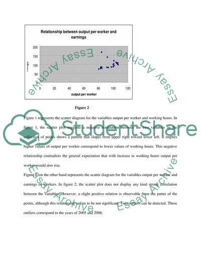
Relationship between Output Per Worker and Working Hours Statistical analysis and results The hypothesis to be tested for the present research is as follows: Null Hypothesis- H0: More working hours and higher earnings lead to a higher output per worker within the mining industry. To test this hypothesis various statistical tool can be used. For example the simplest way to find out the nature of relationship between any two variables is to form a scatter diagram. In the present case, objective are to find out how output per worker in mining industry is related to the amount of working hours and the level of earnings. Here two scatter diagram can be used to find out what kind of correlations exist (I) between output per worker in the mining industry and the number of working hours and (II) between output per worker in the mining industry and the level of income. The two scatter diagrams are presented below: Figure 1 Figure 2 Figure 1 represents the scatter diagram for the variables output per worker and working hours. In figure 1, the scatter plot suggests a negative correlation between the two variables as the collection of points shows a pattern that slopes from upper right toward lower left. It implies higher values of output per worker correspond to lower values of working hours. This negative relationship contradicts the general expectation that with increase in working hours output per worker would also rise. Figure 2, on the other hand represents the scatter diagram for the variables output per worker and earnings of workers. In figure 2, the scatter plot does not display any kind strong correlation between the variables. However, a slight positive relation is observable from the patter of the points, although this relationship seems to be not significant. Two outliers can be detected. These outliers correspond to the years of 2005 and 2006. On the basis of the scatter diagrams presented above, it can be inferred that in both of the cases real life situations do not appropriately match with expectations. To get in depth view regarding the pattern of relationships of the dependent variable, i.e. output per worker with each of the independent variables, i.e. working hours and worker’s earnings, a multiple regression can be run. To run a multiple regression with the help of the data at hand, the following regression equation has to be estimated- yt = α + β1 ht + β2 et + ut ……………………………………………………………………………….(1) In the above equation, yt represents output per worker at period t, ht stand for working hours at period t, et stand for worker’s earnings at period t, and ut is the error term. β1 is the coefficient of the variable working hours. The sign of this coefficient represents the direction of the effect of working hours on output per worker, while its magnitude reflects the extent by which output per worker is affected by working hours. Similarly β2 is the coefficient of the variable worker’s earnings. The sign of this coefficient represents the direction of the effect of worker’s earnings on output per worker, while its magnitude reflects the extent by which output per worker is affected by working hours. (Allison, p. 41; Berk, pp.103-105) Equation 1 is a multiple regression model. In terms of the coefficients in the regression equation 1, the hypothesis that is going to be tested can restated as follows: β1> 0 and β2 >0. To test this hypothesis, one needs to solve the regression equation stated above. To solve regression equation (1) ordinary least square method can be applied. It is one of the convenient methods of running regression. The objectives are to determine the estimated values of α, β1, and β2. The estimated values of the parameters can be denoted by α^, β1^, and β2^. Solving equation 1 by applying ordinary least square technique, the values of α^, β1^, and β2^ can be obtained and these values can be expressed as follows: α^ = y* - β1^ h* - β2 ^e* , where y*, h*, and e* are the mean values of the variables y, h, and e and β1^ = (S22S1y – S12S2y)/ (S11S22 – S122); and β2^ = (S11S2y – S12S1y)/ (S11S22 – S122) Here, S11 = ∑ (ht2) – n h*; S22 = ∑ (et2) – n e*; S1y = ∑ (ht yt )– n h*y*; S2y = ∑ (et yt )– n e*y*; S12 = ∑ (et ht )– n e*h*. (Allison, pp 41; Berk, 103-105) After running the regression using the data at hand, the following results have been obtained. Table 1 presents the results of multiple regression analysis. In Table one, it can be seen that the value of R2 is very high. In multiple regression analysis R2 is called the coefficient of multiple determination. It actually shows how much of the variation in the values of the dependent variable in the sample can be explained by the variation in the values of explanatory variables in the sample. The value of R2 lies in the range of 0 to 1. If the value of R2 is closed to 1, then it can be said that most of the variations in the values of the dependent variable in the sample can be explained by the variation in the values of the independent variables. Opposite is the case if R2 is found to be lying near 0, i.e. if the values of R2 lies near 0, it can be said that variations in the values of the explanatory variables taken under consideration in the regression analysis is not sufficient enough to account for the variations in the values of the dependent variable in the regression analysis. Here R2 in the estimated multiple regression equation is equal to 0.90 (approximately). It implies that around 90 percent of the variations in the values of the output per capita, which is the dependent variable in the present problem, can be explained by the variation in the values of the independent variables working hours and worker’s earnings. From the value of the R2, one thing has become quite clear that output per capita in the mining industry quite significantly dependent on working hours and worker’s earnings. However, only on the basis of the value of R2, it would not be possible here to draw any conclusion. To make a decision regarding the acceptance or rejection of the hypothesis under consideration, it is necessary to look at the sign and the values of the coefficients in the results that have been obtained by estimating the regression with multiple explanatory variables. (Allison, pp 41; Berk, 103-105) In table 1, it can be found that the coefficient of working hours, i.e. β1, and the coefficient of worker’s earnings, i.e. β2, both have negative sign. From the results, β1 is found to be equal to (-0.86) approximately, while β2 is found to be equal to (-0.09) approximately. Hence, it becomes quite clear that working hours of the workers in the mining industry is far more important than the earnings of workers in the determination of the level of output as the coefficient of working hours is found to be quite larger than the value of the coefficient of worker’s earnings. The values of these coefficients say that if working hours is increased by one unit, then the output level will be decreased by far greater extent than when earning of worker is increased by one unit. It can be said that said that when working hours is increased by 1 unit, output per worker is decreased by 0.86 unit. But when worker’s earning is increased by 1 unit, then output per capita is decreased by only 0.09 units. So it can be said that working hours are far more influential than workers earning. However, the relationship between output per capita and the relationship between output per capita and worker’s earning are found to contradict general expectation. On the basis of above analysis of the results, time has, however, not come to make any decision. To find out whether the hypothesis holds for the present sample, it is necessary to conduct t test. On the basis of the t test it can be said whether the values of the coefficients obtained through regression by employing OLS are statistically significant or not. In the present case if the t ratios of the coefficients are found to be statistically significant then null hypothesis will be rejected. Now the t ratios for the present regression analysis can be presented as follows: t ratio for the coefficient of ht is : (β1^)/ Standard error (β1) and t ratio for the coefficient of et is : (β2^)/ Standard error (β2). (Allison, pp 41; Berk, 103-105) Table 1 presents the values of the t ratios for the present problem. Here, t ratio for β1 is equal to (-12.06) approximately. Now with degrees of freedom 17 (since number of observations are 20, and number of parameters are 3 including the intercept term), at the 5 percent level of significance, probability points are (+-) 2.110 with a two-tailed test. In any statistical test on the basis of t ratio, a hypothesis is rejected when the observed value of t ratio is found to be greater than (+) tabulated value of the t ratio or smaller than (-) the tabulated value of the t ratio that are given in the t table. In the present case the observed or calculated value of the t ratio of coefficient β1 is less than -2.110. Therefore, it can be said that the coefficient is statistically significant and hence the hypothesis that β1>0 will be rejected as the estimated value of the coefficient has already found to be less than zero. On the other hand, t ratio for β1 is equal to (-2.64) approximately. Now since with degrees of freedom 17 (since number of observations are 20, and number of parameters are 3 including the intercept term), at the 5 percent level of significance, probability points are (+) 2.110 and (-) 2.110 with a two tailed test, the hypothesis that β2>0 will be rejected as observed value of the t ratio of β2, i.e. -2.64 is less than -2.110. Therefore, it can be said that the coefficient is statistically significant and hence the hypothesis that β2>0 will be rejected as the estimated value of the coefficient has already found to be less than zero. To confirm the results obtained through multiple regression analysis, two single regressions have also been run. In the first single regression independent variable is working hours and in the second equation the independent variable is worker’s earnings. Table 2 and table 3 present the results of these two single regressions. Looking at the results presented at table two, it can be said that working hours, when considered alone, significantly affects output per worker, but in a negative way. On the other hand, in table 2 it is seen that unlike in case of multiple regression analysis, when earning of worker is considered to be the sole independent variable, then the coefficient become positive. But the important thing to be noted here is that in spite of showing a positive relation with output per capita, the effect of worker’s earning on output per capita is very low and statistically insignificant. Since the obtained results appear to contradict general expectation, it would be wiser to examine whether the given sample violate any assumptions that are required for performing regression using Ordinary Least Square method. Here, it is now necessary to check for heteroskedasticity and multicollinearity. The term Heteroskedasticity stands for absence of a common variance of the error terms. Multicollinearity, on the other hand, implies that explanatory variables in the regreaaion analysis are intercorrelated. Since, the sample used for the present study is not very large, Goldfeld and Quandt Test can be applied. In case of Goldfeld and Quandt Test, the observations in the sample is split into two groups- one group corresponding to large values of one explanatory variable and the other group corresponding to small values of the same explanatory variable. The middle most observations are not taken under consideration. Separate regressions are run for each group and then F statistic is calculates. In the present case, the first group corresponds to higher values of worker hours and the second group corresponds to lower values of worker hours. Each group consists of seven observations under each variable. Running regressions separately for each set of observation it is found that standard errors for the first and second sets of observations are 1.31 and 2.44 (approximately), respectively. Therefore F ratio is: F= 2.44/1.31 = 1.87 Now the 1 percent point for the F distribution with degrees of freedom 4 and 4 is 6.39. thus the F value is not significant at 1 percent level and it can be concluded that the error terms for the present sample are homoskadastic, i.e. have a common variance. Therefore, in the present case there is no problem of heteroskadasticity. Now, to check for multicollinearity, a simple rule of thumb can be used. By Klein’s rule there would exist the problem of multicollinearity if the squared multiple correlation coefficient between the dependent and independent variables is smaller than squared multiple correlation coefficient of one explanatory variable with the other explanatory variables. Here, squared multiple correlation coefficient between the dependent and independent variables is equal to 0.67 and squared multiple correlation coefficient of one explanatory variable with the other explanatory variable is 0.81. It simply implies that multicollinearity problem exists in the present case. This also seems quite logical because workers earnings depend on number of working hours. As number of working hours rises, income also rises. In the presence of multicollinearity, it becomes quite difficult to disentangle separate effect of each explanatory variable on dependent variable. Therefore, the results that are obtained by running regression in presence of multicollinearity do not reflect appropriate picture. So, it becomes quite difficult to draw conclusion in presence of multicollinearity. The unexpected results in the present case can also be attributed to the fact that a number of variables that have potential to influence output have been omitted from analysis. For example, factors like changing demand for coal, application of new technologies that increases productivity, and the degree of trade unionization in the mining industry have huge potential to increase output. These factors are capable enough to affect the level of output irrespective of the change in the level of working hours or worker’s earnings. So, there exists a possibility that these factors might be highly effective in mining sector and therefore irrespective of the direction of changes in the number of working hours and worker’s earning have made output per worker to increase. Table 1: results of the multiple regression, where output per worker has been regressed two independent variables - over working hours and workers earning SUMMARY OUTPUT Regression Statistics Multiple R 0.948149 R Square 0.898987 Adjusted R Square 0.887103 Standard Error 3.083698 Observations 20 ANOVA   df SS MS F Significance F Regression 2 1438.693 719.3466 75.6475 3.45E-09 Residual 17 161.6563 9.509192 Total 19 1600.349         Coefficients Standard Error t Stat P-value Lower 95% Upper 95% Lower 95.0% Upper 95.0% Intercept 188.5978 8.929368 21.12107 1.2E-13 169.7585 207.4371 169.7585 207.4371 Working hours (ht) -0.8574 0.071111 -12.0573 9.4E-10 -1.00743 -0.70737 -1.00743 -0.70737 Earnings ( et) -0.08943 0.033826 -2.64378 0.01706 -0.16079 -0.01806 -0.16079 -0.01806 Table 2: results of the multiple regressions, where output per worker has been regressed over working hours. SUMMARY OUTPUT Regression Statistics Multiple R 0.925989 R Square 0.857455 Adjusted R Square 0.849536 Standard Error 3.559974 Observations 20 ANOVA   df SS MS F Significance F Regression 1 1372.228 1372.228 108.27613 4.82709E-09 Residual 18 228.1214 12.67341 Total 19 1600.349         Coefficients Standard Error t Stat P-value Lower 95% Upper 95% Lower 95.0% Upper 95.0% Intercept 172.2599 7.440985 23.15015 7.605E-15 156.6269561 187.8928 156.627 187.8928 Working hours (ht) -0.78148 0.075102 -10.4056 4.827E-09 -0.939261983 -0.6237 -0.93926 -0.6237 Table 3: results of the multiple regression, where output per worker has been regressed over worker’s earnings. SUMMARY OUTPUT Regression Statistics Multiple R 0.187516 R Square 0.035162 Adjusted R Square -0.01844 Standard Error 9.261863 Observations 20 ANOVA   df SS MS F Significance F Regression 1 56.27163 56.27163 0.655983 0.42856 Residual 18 1544.078 85.7821 Total 19 1600.349         Coefficients Standard Error t Stat P-value Lower 95% Upper 95% Lower 95.0% Upper 95.0% Intercept 87.81949 9.437001 9.305868 2.67E-08 67.99308 107.6459 67.993082 107.6458891 Earnings (et) 0.075276 0.092942 0.809928 0.42856 -0.11999 0.27054 -0.1199874 0.27053986 Table 4: Regression output of first set of observations of Goldfeld-Quandt Test SUMMARY OUTPUT Regression Statistics Multiple R 0.896515 R Square 0.80374 Adjusted R Square 0.70561 Standard Error 1.306575 Observations 7 ANOVA   df SS MS F Significance F Regression 2 27.96484 13.98242 8.190556 0.038518 Residual 4 6.828556 1.707139 Total 6 34.79339         Coefficients Standard Error t Stat P-value Lower 95% Upper 95% Lower 95.0% Upper 95.0% Intercept 166.2559 15.65512 10.61991 0.000445 122.7903 209.7215 122.7903 209.7215 X Variable 1 -0.48049 0.120842 -3.9762 0.016453 -0.81601 -0.14498 -0.81601 -0.14498 X Variable 2 -0.18976 0.068665 -2.76356 0.050664 -0.38041 0.000885 -0.38041 0.000885 Table 5: Regression output of second set of observations of Goldfeld-Quandt Test SUMMARY OUTPUT Regression Statistics Multiple R 0.819604 R Square 0.67175 Adjusted R Square 0.507626 1.869516 Standard Error 2.442663 Observations 7 ANOVA   df SS MS F Significance F Regression 2 48.84171 24.42085 4.092925 0.107748 Residual 4 23.86641 5.966602 Total 6 72.70812         Coefficients Standard Error t Stat P-value Lower 95% Upper 95% Lower 95.0% Upper 95.0% Intercept 165.7593 28.79528 5.756477 0.004517 85.81083 245.7078 85.81083 245.7078 X Variable 1 -0.69389 0.24298 -2.85574 0.046128 -1.36851 -0.01927 -1.36851 -0.01927 X Variable 2 -0.0499 0.035892 -1.39031 0.236798 -0.14955 0.049752 -0.14955 0.049752 References 1. Allison, Paul David Multiple regression: a primer. Pine Forge Press, 1999. 41 to 45 2. Berk, Richard A. Regression Analysis: A Constructive Critique. London: Sage. 2003 3. Gomez, Arturo A. Statistical Procedures for Agricultural Research. IRRI. 1984. 398 Read More