Phillips Curve and Unemployment - Inflation Dilemma for Policy Makers - Coursework Example

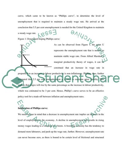
Phillips Curve and Unemployment - Inflation Dilemma for Policy Makers Introduction: Unemployment rate is a distinct macro indicator, which is utilised to assess the performance of an economy. By trying to cull out the major causes responsible for unemployment, Mankiw (2007) points out that the natural rate of unemployment depends on a number of factors, such as minimum wage laws, strength of the labour union, efficiency of wages, effectiveness of job search, etc. The rate of inflation is another important measure of economic performance. Classical economic theory, particularly Irwin Fisher’s equation of exchange, empahsises that inflation rate depends on excessive growth of money supply in the economy. Thus, although unemployment and inflation appear to be unrelated issues, Phillips curve establishes the linkage between the two, with empirical evidence. A.W. Phillips (1958) in an article titled, “The relationship between unemployment and the rate of change of money wages in the united kingdom, 1861-1957”, captures the dynamic linkage between inflation and unemployment. Historical Development: A.W. Phillips (1958) made an empirical study on the relationship between the rate of unemployment and the rate of change in money wages in the United Kingdom, for the period between 1861 and 1957. He was of the view that rate of changes in money wages can be explained by the level of unemployment in an economy. He set out to enquire if statistical evidence will support such a hypothesis. Phillips found that there is a negative relation between unemployment and the rate of change in money wages. Armed with his findings, Phillips used this downward slopping curve, which came to be known as “Phillips curve”, to determine the level of unemployment that is required to maintain a steady wage rate. He arrived at the conclusion that 5.5 per cent unemployment is needed for the United Kingdom to maintain a steady wage rate. Figure 1: Downward sloping Phillips curve: As can be observed from Figure 1, the point U represents the unemployment rate that is needed to maintain stable wage rate. From Alfred Marshall’s marginal productivity theory of wages, it can be construed that an increase in wage rate in proportion to an increase in labour productivity is non-inflationary. Phillips, thus, further estimated that 2.5 per cent unemployment is a must to maintain price stability. This implies that wages will rise by the same percentage as the increase in labour productivity, which was estimated to be 3 per cent. Hence, Phillip’s curve serves to be an effective policy tool for a trade-off between inflation and unemployment rates. Implication of Phillips curve: We need to bear in mind that a decrease in unemployment rate implies an increase in the level of employment in the economy. A decline in unemployment rate results in rising money wages leading to a situation of a boom. A booming economy has the tendency to demand more labourers, and push up the wage rate, further. However, unemployment rate can never become zero, as there is bound to be certain level of frictional and structural unemployment. Alternatively, at high unemployment level, i.e. at the lower portion of the Phillips curve, wage inflation remains unresponsive to changes in unemployment rate (Lipsey and Chrystal, 1995). Later Developments: Samuelson and Solow (1960) estimated a similar curve for the United States. They painted a more gloomy picture of the American economy by concluding that an unemployment rate of 5.5 per cent is necessary for price stability in the United States, with an assumption that labour productivity increased by 2.5 per cent, annually. Thus, Samuelson and Solow (1960), and later Lipsey (1960) propagated the Phillips curve as an instrument of economic policy. They substituted the variable w, which represents money wages, for ∏, which presents the rate of inflation. They argued that if labour productivity increased by 2 per cent per annum, then a 2 per cent increase in money wages will be non-inflationary. Hence they pointed out that a trade-off exists between the rate of inflation and the unemployment rate, so that the government has the possibility of choosing alternative points on the Phillips curve with different rates of inflation and unemployment. One of the important implications of this trade-off is that inflation and unemployment can co-exist; and they are not mutually exclusive events (Makinen, 1978). The experience of many developed countries shows that as unemployment is reduced below a certain critical level, prices begin to rise. Therefore, the choice lies with the policy makers. If the policy makers feel the need to stabilize the price level, then the economy has to let go a high level of employment. Alternatively, if the policy makers choose to achieve a high level of employment, it will be at the expense of stable prices. This implies that there is a trade off between unemployment and inflation. Does the Theory Fit the Facts? This study deals with two sets of data pertaining to two imaginative countries, A and B. An analysis of the data sets involving inflation and unemployment rates for the imaginative two countries, A and B, provides certain interesting results. Data sets of Imaginative Country B: Figure 2: Scatter Plot for country B: As can be observed from Figure 2, the downward sloping straight line represents the Phillips curve which establishes the relationship between the rate of change in inflation rate and unemployment where the inflation rate is depicted on the y axis, and the percentage of unemployment on the x axis. The Phillips curve indicates that as unemployment reaches approximately 9.5 per cent, inflation rate remains zero. Any effort by the policy makers in country B to reduce unemployment rate will result in inflation. Thus for the imaginative country B, Phillips curve becomes an effective policy instrument for a trade-off between unemployment and inflation. If we consider a regression model for the imaginative country B, then the model can be written as ∏ = α + β (Unemployment rate) +μ where ∏ represents the inflation rate, α represents the intercept, β the slope and μ the error term. Table 1: Model Summary for the Imaginative Country B: R R Square Adjusted R Square Std. Error of the Estimate 0.879 0.773 0.766 1.00 As there is only one independent variable, unemployment, R value of 0.879 represents the simple correlation between inflation and unemployment. The R2 value of 0.773 indicates that the 77 per cent of the variation in inflation is explained by unemployment. Thus, this R2 value represents a sound measure of goodness of fit in the model. The adjusted R2 value of 0.766 is significant, and it reflects how well the model fits the population. Table 2: Analysis of Variance (ANOVA) for the Imaginative Country B: Sum of Squares df Mean Square F Sig. Regression 110.855 1 110.855 109.177 .000 Residual 32.492 32 1.015 Total 143.347 33 The F statistics of 109.177 is used to test the hypothesis that the slope of β is zero. As can be observed from the ANOVA table, below, the linear relationship between inflation and unemployment is highly significant as the p value of F is less than 0.0005. Table 3: Coefficients of the model for the Imaginative Country B: Coefficients Unstandardized Coefficients Standardized Coefficients t Sig. B Std. Error Beta (Constant) 6.935 0.388 17.888 0.000 Unemployment in B -0.665 0.064 -0.879 -10.449 0.000 As can be observed from the coefficients: The estimates of the model coefficients, α = 6.935, and the slope is -0.665. Thus, the estimated model is 6.935 – (0.665 x unemployment rate) Freidman (1968) and Phelps (1967) do not agree with the trade-off theory of A.W. Phillips, and point out that in the long run, Phillips curve does not exist. Even if it does, then it will not be a downward sloping one, but at best a vertical straight line. Data Sets of Imaginative Country A: Figure 3: Scatter Plot for Country A: This scatter plot for country A indicates that the data set is not useful to explain the trade-off between inflation and unemployment rates. As can be observed from this figure, inflation and unemployment rates in the imaginative country are two different disconnected variables. Hence, empirical evidence of Philip’s curve remains an issue of controversy. Some economists are of the view that changes in prices are equally important as unemployment in determining wage rate. Thus they conclude that Phillips curve does not adequately lend itself to macroeconomic decision making. Harry Johnson (1969) argues that Phillips curve represents only a statistical description of the mechanics of adjustment in the labour market, and thus he doubts its applicability at specific point of time in any economic activity. Data set for the imaginative country A appears to be a good fodder for Friedman and Phelps. Friedman (1968) and Phelps (1967) argue that Phillips curve exists only in the short run, and they insist that the so-called downward sloping Phillips curve does not exist in the long run, and consequently there is no trade-off between inflation and unemployment. They base their argument on adjustment in people’s expectation. They point out that as soon as inflation begins to rise, people expect the prices to increase. People realise that the increased money wages will be wiped out by the increase in inflation. Thus the economy is faced with a higher level of inflation coupled with the same level of unemployment. Hence, Phillips curve can be a vertical straight line, in the long run, as in the case of the data pertaining to the imaginative country A. Since the 1960s, a number of econometric studies were undertaken to find Phillips curve for different countries. In the process, Perry (1966) added other variables such as price index and profit rates to the inflation rate. Similarly, Hines (1972) considered the degree of unionization as an additional cost-push component. Makinen (1978) elaborated on the slope and position of the Phillips curve, which are crucial to determine the socially tolerable levels of inflation and unemployment. Conclusion: We looked at the origin and development of Phillips curve. We utilised the data sets pertaining to two imaginative countries to test the applicability of Phillips curve. While the imaginative country B supports the findings of A.W. Phillips, the data sets of country A indicate that there are other exogenous variables, which may determine the inflation rate. In such a situation, it may not be simple enough to establish the association between unemployment and inflation. Thus, we can conclude that despite the disagreement among the scholars in using Phillips curve as a powerful policy tool, Phillips curve approach remains very much relevant to countries to choose between the various combinations of unemployment and inflation rates. **** Abstract: Since the 1960s, Phillips curve has become an important policy tool to choose between unemployment and inflation rates. Evidence indicates that many counties around the world have utilised Phillips curve to arrive at their policy option. However, Friedman and Phelps contest the usefulness of Phillips curve as a trade-off between unemployment and inflation, in the long run. We fitted two data sets pertaining to two imaginative countries, in this study. The results indicate that Phillips curve is valid and reliable in the case of imaginative country B. This study also finds that there may be other exogenous factors which come in the way of the association between unemployment and inflation, as in the case of imaginative country A. Appendix: Regression results for the imaginative country A: Model Summary R R Square Adjusted R Square Std. Error of the Estimate .389 .151 .125 2.3905 ANOVA Sum of Squares df Mean Square F Sig. Regression 32.594 1 32.594 5.703 .023 Residual 182.870 32 5.715 Total 215.464 33 a Predictors: (Constant), UNEMP_A b Dependent Variable: INFLA_A Coefficients Unstandardized Coefficients Standardized Coefficients t Sig. B Std. Error Beta (Constant) -.244 1.924 -.127 .900 UNEMP_A .717 .300 .389 2.388 .023 a Dependent Variable: INFLA_A Comments on your earlier Graphs: Country A My Comments: 1. An increase in inflation rate in country A leads to an increase in unemployment rate, with a time lag, and vice versa. 2. An increase or decrease in inflation rate precedes the increase or decrease in unemployment rate. 3. There seems to be a causal relationship between the two variables, just as in the case of Milton Friedman’s thesis on relationship between money supply and trade cycle or fluctuations in the economy. 4. During the initial years, the interaction between the two variables is much closer as compared with later years, i.e. from the 12th year onwards. 5. The deviation between the two variables are marginal for the first 11 years (Standard deviation = 1.5), while it is significant (Standard deviation = 2.3) after the 12th year. 6. The gap between the two variables becomes narrow between 20th and 22nd year, as well as between 31st and 32nd years. Country B: My Comments: 1. Both inflation and unemployment rates for country B are two strong opponent factors. 2. With minor variations, if one factor increases, the other factor decreases and vice versa. 3. Their negative relationship can be captured by their correlation coefficient. The correlation between the two variables for the entire period is = -0.879, which is very significant to prove the point that their relationship is negative, almost to the perfection. 4. Standard deviation between the two variables during the first two years is estimated at 4.1, during 15th and 16th years it accounts for 2.9, and during 30th to 34th year it is 3.8 5. The meeting points of the two variables are 7th, 12th and the 22nd years, as the standard deviation for these years remain at 0.21, each, during these years. References: Friedman, Milton. 1968, “The Role of Monetary Policy”, American Economic Review, No. 58, pp.1-17. Harry G. Johnson. 1969, “Essays in Monetary Policy”, American Economic Review. Hines, A.G. 1972, The Phillips Curve and the Distribution of Unemployment, The American Economic Review, Vol. 62, No. 1 / 2 , pp. 155-160. Lipsey G. Richard. 1960, “The Relation between Unemployment and the Rate of Changes in Money Wage Rates in the United Kingdom, 1862-1957: A Further Analysis”, Economica, No. 27, pp.1-31. Lipsey, G. Richard and K. Alec Chrystal. 1995, An Introduction to Positive Economics, 8th edition, University Press, Walton Street, Oxford. Makinen E. Gail. 1978, Money, the Price Level, and Interest Rates: An Introduction to Monetary Theory, Prentice-Hall of India Private Limited, New Delhi. Mankiw, N. Gregory. 2007, Principles of Macroeconomics, 4th Edition, Harvard University, Thomson, South-Western. Perry, L. George. 1966, Unemployment, Money Wage Rates and Inflation, Cambridge: The MIT Press. Phelps, S. Edmund. 1967, “Money Wage Dynamics and Labour Market Equilibrium”, Journal of Political Economy, pp. 678-711. Phillips, A.William. 1958, “The Relationship between Unemployment and the Rate of Change of Money Wages in the United Kingdom”, Economica, No. 25, pp. 283-299. Samuelson, Paul A., and Robert M. Solow. 1960, “Analytical Aspects of Anti-inflation Policy” American Economic Review, 50, No.2, pp.177-94. Read More