Quantitative Finance - Admission/Application Essay Example

Solution 1. = Where C is the price of a call, P the price of a put, K the strike-price of the options, So the price of the stock at time zero, S the price of the stock at maturity, T the time to maturity, and rf the risk free rate. =, So = 91.3162 It is always hard for retail traders to get in the arbitrage, but that does not mean that its principles can’t be used in away to get more of the available trades to expire. Though it is not a strategy but much of a technique you can as well develop a great strategy from it by making currency demand of currency high so that its value can be increased as well.

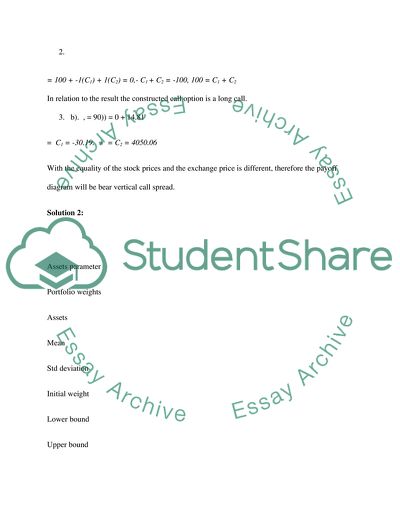
Using the relative value of currencies between their pairs can give you some insight into where the market might be going. c). minimum profit of strategy = strike price of long call – strike price of lower long call + net premium – commission paid = $100 - $4 - $(3% of 95) = $93.15 2. = 100 + -1(C1) + 1(C2) = 0,- C1 + C2 = -100, 100 = C1 + C2 In relation to the result the constructed call option is a long call. 3. b). , = 90)) = 0 + 14.81 = C1 = -30.19. = = C2 = 4050.06 With the equality of the stock prices and the exchange price is different, therefore the payoff diagram will be bear vertical call spread.

Solution 2: Assets parameter Portfolio weights Assets Mean Std deviation Initial weight Lower bound Upper bound A 0.3533 0.4573 0.04 0.02 1 B 0.3667 0.4485 0.08 0.02 1 C 0.495 0.38997 0.12 0.5 1 D 0.4833 0.3704 0.15 0.3 1 Assets Assets| A B C D A 1.000 B -1 1.000 C 1 1 1.000 D -1 -1 1 1.000 1. Ʃ = SRS, where S is a diagonal matrix for standard deviation. = 0.4896 2. , = = =0.4896 µ - 0.04896 = 0, µ = = 0.1 b). the most important is the first moment given by: Where, µn = Rn = = 231.

46522E + 0.1EP = 17.4034 , = 231.56522E = The portfolio risk of return is quantified by ð2p in mean-variance analysis, only the first moments are considered in the portfolio model. Investment theory prior to Markowitz considered the maximization of µp but without ðp The mean portfolio is zero since at time zero the tangency portfolio is absolute zero. 3. X = X = X = 0.2037 F = 0.033 N/B: Notice that variance of the portfolio return depends on three variance terms and six covariance terms.

Hence, with four assets there are twice as many covariance terms than variance terms contributing to portfolio variance. Works Cited Day, R. A., and A. L. Underwood. Quantitative analysis. 2d ed. Englewood Cliffs, N.J.: Prentice-Hall, 1967. Print. Quantitative finance. Bristol, UK: Institute of Physics Pub., in association with American Institute of Physics, 2001. Print.