Dynamic Programming: Resource Allocation - Assignment Example

Executive summery: Dynamic programming approach usually offers an optimal solution for complex reservoir operational problems. In this report analysis an attempt to determine the relevance of the dynamic programming in resource allocation scenario as one of the optimizing tool to be relied upon in making decision. A brief overview will include its application, advantages and its shortfalls as well. The final result of module formulation shows the applicability of the dynamic programming in resolving the investment decision.

Introduction: The report describes how to formulate and implement by allocating resources using a dynamic programming. The method allows the fund manager to make an informed decision of investing the $10 million on behalf of the pension fund. In addition, it shows the optimal return expected to be earned at different risk levels. The results are tested and confirm through formulating different stages for each product through a simplified scenario. The investment details are illustrated using the scenario bellow.

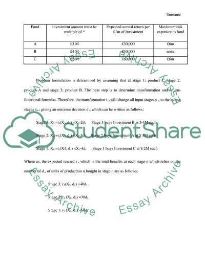
Fund Investment amount must be multiple of * Expected annual return per £1m of investment Maximum risk exposure to fund A £3 M £30,000 £6m B £4 M £40,000 none C £2 M £60,000 £6m Problem formulation is determined by assuming that at stage 1; product C, stage 2; product A and stage 3; product B. The next step is to determine transformation and returns functional formulas. Therefore, the transformation t n will change all input stages x n to the output stages xn-1 giving an outcome decision d n which can be written as follows; Stage 3: X2 =t3(X3, d3) =X3-2d3 Stage 3 buys Investment B at $ 4M each Stage 2: X1 =t2(X2, d2) =X2-3d2 Stage 2 buys Investment A at $ 3M each Stage 1: X0 =t1(X1, d1) =X1-4d1 Stage 1 buys Investment C at $ 2M each Where as, the expected reward r n which is the total benefits at each stage n which relies on the number of d n of units of production n bought in stage n are as follows; Stage 3: r3(X3, d2) =40d3 Stage 2: r2 (X2, d2) =30d2 Stage 1: r1 (X1, d1) =60d1 The objective function i.e. the total return from investment at this initial stage includes only the total reward r 1 as there is no any other previous stage.

Therefore the output as well as the objective function is determined as follows: X 0 = X1-4d1; f1 (X1) = r1(X1, d1) = 60 d1 Where 0 ≤ X 1 ≤ 9 and 0 ≤ d1≤ (Appendix table 1) X1 shows the input at stage 1, d1 is the anticipated decisions at this particular stage, where as, d*1 is the optimal decision at a given value of input X1 and f1(x1) is the reward to be earned for making decision d1 using input X1. At stage 2, the decision d2 is the number of units purchases for product C such that 0 ≤ d2≤ 1(Appendix table 2).

The output at this stage is X1=X2-3d2 and the objective function is F2(X2) =30d2+f1(X1) where f1(X1) represents the exact value of objective function calculated in the previous stage. At stage 3 (product B $ 4 M $40K), is the stage where the investment is at its maximum i.e. the value of X3= 9 the result at this stage is as shown in table 3. Where the optimal results are; Stage 3: X3 = 9, d3=1, X2=X3-2d3=9-2=7 Stage 2: X2=7, d2=1, X1=X2-3d2=7-3=4 Stage 1: X1=4, d1=1, X0=X1-4d1=4-4=0 (Appendix table 3).

According to the results it shows that the fund manager should consider purchasing the following Stage 3: One unit of product C at a cost of 2 millions Stage 2: One unit of product A at a cost of 3 millions Stage 1: One unit of product B at a cost of 4 millions This will optimize the investment i.e. 2+3+4+9 Millions and the expected returns will be $60,000 per unit of $ 1 million investment from product C $30,000 per unit of $ 1 million investment from product A $40, 000 per unit of $ 1 million investment from product B Thus, the total returns will be $ 190 millions which is the same as the value of the objective function in stage 3 Conclusion: Based on the above results, it is quite clear that, unlike linear programming, dynamic programming is very simple to formulate and solve since there are no complex variables.

In addition, the incorporation of different constraints is much easier as compared to linear and non linear programming. Thought that is the case, there are some disadvantages of this method, for instance, designing and formulating the recursive equations may be so frustrating and complex beside not providing one time period solution to various problems as compared to linear programming. Therefore, considering all the above, the manager would be in a better position in making the investment decision using dynamic programming.

Appendix 1 Table 1   d1   X1 0 1 2 d*1 F*1(x1) x0 0 0     0 0 0 1 0     0 0 1 2 0     0 0 2 3 0     0 0 2 4 0 60   1 60 0 5 0 60   1 60 1 6 0 60   1 60 1 7 0 60   1 60 3 8 0 60 120 2 120 0 9 0 60 120 2 120 1 Table 2 d2   X2 1 2 d*2 f2(x2) x1 0 0   0 0 0 1 0   0 0 0 2 0   0 0 0 3 0 30 1 30 0 4 60 90 1 90 1 5 60 90 1 90 1 6 60 90 1 90 3 7 60 90 1 90 4 8 120 150 1 150 5 9 120 150 1 150 6 Table 3       d3       X3 0 1 2 3 4 5 6 d*3 f3(x3) X2 9 150 190 150 100 120 150 180 1 190 7 References: Bellman, Richard, 1957, “Dynamic Programming” Princeton, NJ: Princeton University Press.

Breton, Michele, Pascal & Francisco 2006, Dynamic programming approach to price installation option, “European Journal of operational Research, Vol. 169(2), pages 667-676. Elton, Edwin, J, & Gruber, Martin J, 1971, “Dynamic Programming Approach to price installment in Finance, “Journal of Finance, Vol. 26(2), pages 473-506 Finn E, & Edward C. Prescott, 1977, “Rules rather than the discretion: The Inconsistency Dynamics” Cambridge, MA: Harvard University Press, 198 George G, Rogers, David F, Sweeney & Dennis J, 2010, “Risk management strategies of portfolio optimization,” Euro Journal of operation Research, Vol. 207(1), page 409-419 Handy, A, Tasha, 2006, “Operational research; Introduction, eighth edition, prentice, hall in India private limited, New Delhi James C, T, Mao & Carl E, S, 1966, “Decision Theory Approach to portfolio selection” Management science, Vol. 12 (8), page B323-B333.

Martin R, & Young, 1998, “A minim ax portfolio selection rule with lines Linear Programming solution” Management Science, Vol. 12(8), page B323-B333. Nancy, Robert E, Lucas, Edward C. & Prescott, 2009, “Recursive methods in economic Of optimal plans," Journal of Political Economy, 1977, 85, 473-491 Sharma, J, K, 2007, Operational research; Theory and application, third edition, Macmillan publishers