The Application of ANOVA to Baseball Team Parameters - Research Paper Example

The Application of ANOVA to Baseball Team Parameters SCHOOL Table of Contents I. Research Question We pose the research question as: to what extent is attendance at games a function of salaries and winning record? The rationale for this research question is that baseball fans are more likely to watch teams that win more consistently and are top-heavy with stars (implied by the high salary level of the team). Hence: Attendance = f (Salaries, Wins) II. The Applicable Hypotheses Given the definition of the ANOVA model in the succeeding section, the hypotheses can be articulated as: Factor Null Alternate A = Team Salary H10 = A1 = A2 = A3…A30 Salary has no effect H11 = Not all Aj are equal to zero Salary has an effect on attendance B = Wins H20 = B1 = B2 = B3…B30 Winning record has no effect H11 = Not all Bj are equal to zero Winning record has an effect on attendance III. The Decision Rule The above research question and hypotheses suggest a two-factor ANOVA model, such that: Y = µ + X1 + X2 + Έ Where: Y = attendance in headcount. X1 = effect of team salary size X2 = effect of winning rate, expressed in the database as a percentage of games won Έ = random error, all other sources of variance not accounted for by X1 + X2. 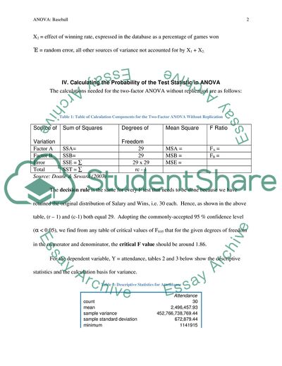IV. Calculating the Probability of the Test Statistic in ANOVA The calculations needed for the two-factor ANOVA without replication are as follows: Table 1: Table of Calculation Components for the Two-Factor ANOVA Without Replication Source of Variation Sum of Squares Degrees of Freedom Mean Square F Ratio Factor A SSA= 29 MSA = FA = Factor B SSB= 29 MSB = FB = Error SSE = ∑ 29 x 29 MSE = Total SST = ∑ rc - 1 Source: Doane & Seward (2007) The decision rule is the same for every F test that needs to be done because we have retained the original distribution of Salary and Wins, i.e. 30 each. Hence, as shown in the above table, (r – 1) and (c-1) both equal 29. Adopting the commonly-accepted 95 % confidence level (α < 0.05), we find from any table of critical values of F0.05 that for the given degrees of freedom in the numerator and denominator, the critical F value should be around 1.86. For the dependent variable, Y = attendance, tables 2 and 3 below show the descriptive statistics and the calculation basis for variance. Table 2: Descriptive Statistics for Attendance   Attendance count 30 mean 2,496,457.93 sample variance 452,766,738,769.44 sample standard deviation 672,879.44 minimum 1141915 maximum 4090440 range 2948525 sum 74,893,738.00 sum of squares 200,099,301,811,402.00 deviation sum of squares (SSX) 13,130,235,424,313.90 population variance 437,674,514,143.80 population standard deviation 661,569.73 standard error of the mean 122,850.42 1st quartile 2,017,372.50 median 2,523,081.50 3rd quartile 2,842,735.75 interquartile range 825,363.25 Table 3: Variance for Y, Attendance Team Attendance Y - Ybar (Y - Ybar)2 Boston 2,847,798 351,340 123,439,844,788 New York Yankees 4,090,440 1,593,982 2,540,778,839,481 Oakland 2,108,818 -387,640 150,264,715,330 Baltimore 2,623,904 127,446 16,242,500,758 Los Angles Angels 3,404,636 908,178 824,787,406,829 Cleveland 2,014,220 -482,238 232,553,421,131 Chicago White Sox 2,342,804 -153,654 23,609,530,204 Toronto 2,014,995 -481,463 231,806,552,964 Minnesota 2,034,243 -462,215 213,642,641,515 Tampa Bay 1,141,915 -1,354,543 1,834,786,549,213 Texas 2,525,259 28,801 829,501,633 Detroit 2,024,505 -471,953 222,739,568,136 Seattle 2,724,859 228,401 52,167,048,777 Kansas City 1,371,181 -1,125,277 1,266,248,169,190 Atlanta 2,520,904 24,446 597,610,338 Arizona 2,059,327 -437,131 191,083,449,963 Houston 2,805,060 308,602 95,235,237,608 Cincinnati 1,923,254 -573,204 328,562,745,367 New York Mets 2,827,549 331,091 109,621,296,634 Pittsburgh 1,817,245 -679,213 461,330,204,279 Los Angeles Dodgers 3,603,680 1,107,222 1,225,940,712,295 San Diego 2,869,787 373,329 139,374,594,507 Washington 2,730,352 233,894 54,706,435,981 San Francisco 3,181,020 684,562 468,625,227,683 St Louis 3,542,271 1,045,813 1,093,724,977,383 Florida 1,852,608 -643,850 414,542,732,361 Philadelphia 2,665,304 168,846 28,508,995,354 Milwaukee 2,211,323 -285,135 81,301,928,306 Chicago Cubs 3,100,092 603,634 364,374,090,465 Colorado 1,914,385 -582,073 338,808,895,839 TOTAL     13,130,235,424,314 In turn, the descriptive statistics and variances for the two independent variables are as follows: Table 4: Descriptive Statistics for Team Salary   Salary count 30 mean 73,063,563.267 sample variance 1,171,964,722,279,950.000 sample standard deviation 34,233,970.297 minimum 29679067 maximum 208306817 range 178627750 sum 2,191,906,898.000 sum of squares 194,135,505,262,785,000.000 deviation sum of squares (SSX) 33,986,976,946,118,700.000 population variance 1,132,899,231,537,290.000 population standard deviation 33,658,568.471 standard error of the mean 6,250,239.255 1st quartile 50,292,565.500 median 66,191,416.500 3rd quartile 87,573,983.750 interquartile range 37,281,418.250 Table 5: Variance for Team Salary Team Salary Y - Ybar (Y - Ybar)2 Boston 123505125.0 50441562.0 2,544,351,176,999,840 New York Yankees 208306817.0 135243254.0 18,290,737,752,508,500 Oakland 55425762.0 -17637801.0 311,092,024,115,601 Baltimore 73914333.0 850770.0 723,809,592,900 Los Angles Angels 97725322.0 24661759.0 608,202,356,974,081 Cleveland 41502500.0 -31561063.0 996,100,697,689,969 Chicago White Sox 75178000.0 2114437.0 4,470,843,826,969 Toronto 45719500.0 -27344063.0 747,697,781,347,969 Minnesota 56186000.0 -16877563.0 284,852,132,818,969 Tampa Bay 29679067.0 -43384496.0 1,882,214,493,174,020 Texas 55849000.0 -17214563.0 296,341,179,280,969 Detroit 69092000.0 -3971563.0 15,773,312,662,969 Seattle 87754334.0 14690771.0 215,818,752,574,441 Kansas City 36881000.0 -36182563.0 1,309,177,865,248,970 Atlanta 86457302.0 13393739.0 179,392,244,400,121 Arizona 62329166.0 -10734397.0 115,227,278,953,609 Houston 76799000.0 3735437.0 13,953,489,580,969 Cincinnati 61892583.0 -11170980.0 124,790,794,160,400 New York Mets 101305821.0 28242258.0 797,625,136,938,564 Pittsburgh 38133000.0 -34930563.0 1,220,144,231,496,970 Los Angeles Dodgers 83039000.0 9975437.0 99,509,343,340,969 San Diego 63290833.0 -9772730.0 95,506,251,652,900 Washington 48581500.0 -24482063.0 599,371,408,735,969 San Francisco 90199500.0 17135937.0 293,640,336,867,969 St Louis 92106833.0 19043270.0 362,646,132,292,900 Florida 60408834.0 -12654729.0 160,142,166,063,441 Philadelphia 95522000.0 22458437.0 504,381,392,482,969 Milwaukee 39934833.0 -33128730.0 1,097,512,751,412,900 Chicago Cubs 87032933.0 13969370.0 195,143,298,196,900 Colorado 48155000.0 -24908563.0 620,436,510,724,969 TOTAL     33,986,976,946,118,700 Table 6: Descriptive Statistics for Wins   Wins count 30 mean 81.000 sample variance 117.379 sample standard deviation 10.834 minimum 56 maximum 100 range 44 sum 2,430.000 sum of squares 200,234.000 deviation sum of squares (SSX) 3,404.000 population variance 113.467 population standard deviation 10.652 standard error of the mean 1.978 1st quartile 73.250 median 81.000 3rd quartile 88.750 interquartile range 15.500 mode 95.000 Table 7: Variance for Team Wins Team Wins Y - Ybar (Y - Ybar)2 Boston 95.0 14.0 196 New York Yankees 95.0 14.0 196 Oakland 88.0 7.0 49 Baltimore 74.0 -7.0 49 Los Angles Angels 95.0 14.0 196 Cleveland 93.0 12.0 144 Chicago White Sox 99.0 18.0 324 Toronto 80.0 -1.0 1 Minnesota 83.0 2.0 4 Tampa Bay 67.0 -14.0 196 Texas 79.0 -2.0 4 Detroit 71.0 -10.0 100 Seattle 69.0 -12.0 144 Kansas City 56.0 -25.0 625 Atlanta 90.0 9.0 81 Arizona 77.0 -4.0 16 Houston 89.0 8.0 64 Cincinnati 73.0 -8.0 64 New York Mets 83.0 2.0 4 Pittsburgh 67.0 -14.0 196 Los Angeles Dodgers 71.0 -10.0 100 San Diego 82.0 1.0 1 Washington 81.0 0.0 0 San Francisco 75.0 -6.0 36 St Louis 100.0 19.0 361 Florida 83.0 2.0 4 Philadelphia 88.0 7.0 49 Milwaukee 81.0 0.0 0 Chicago Cubs 79.0 -2.0 4 Colorado 67.0 -14.0 196 TOTAL     3,404 Table 8: Result of Excel ANOVA Run ANOVA Source of Variation SS df MS F P-value F crit Rows 24004.04 29 827.7257 1.793095 0.060805 1.860811 Columns 944.8054 1 944.8054 2.046724 0.163222 4.182964 Error 13386.93 29 461.6184 Total 38335.78 59         V. Conclusion Given the way the analytical table is set up, Table 8 reveals that the F value across columns exceeds the critical value of 1.85; it can be argued that Wins exceeds the critical value and hence, has the significant effect on attendance. Neither p value, however, meets the confidence level α ≤ 0.05. This suggests that a re-sampling of team performance and stadium attendance might yield very different findings. References Doane, D.P. & Seward, L.E. (2007). Applied statistics in business and economics. New York: McGraw-Hill/Irwin. Read More