StudentShare
Contact Us
Sign In / Sign Up for FREE
Search
Go to advanced search...
Free

Quantitative Analysis of Social Research Data Using SPSS - Assignment Example

Cite this document
Summary
This assignment "Quantitative Analysis of Social Research Data Using SPSS" presents the relative position of men and women in Spain, the UK, and Portugal. It is interesting to make these comparisons in the mentioned countries since these countries have totally different cultures and lifestyles…
Download full paper File format: .doc, available for editing
GRAB THE BEST PAPER95.1% of users find it useful
Quantitative Analysis of Social Research Data Using SPSS
Read Text Preview

Extract of sample "Quantitative Analysis of Social Research Data Using SPSS"

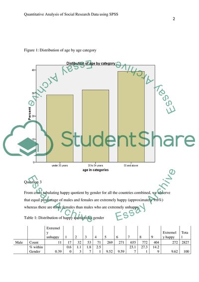
College: Quantitative Analysis of Social Research Data using SPSS Question In this study we are considering relative position of men and women in Spain, United Kingdom and Portugal. It is interesting to make these comparisons in the mentioned countries since these countries have totally different cultures and lifestyles. For this reason we expect to find differences in the way men and women perceive happiness in these countries. Question 2 Continuous age was recoded into a categorical variable named agecat and the categories labelled using the syntax provided in appendix 1. The chart displaying the distribution of age for the three categories is shown in figure 1 below. There were more respondents aged 55 years and above than other age groups. The number of respondents aged below 35 and between 53 and 54 were almost equal. Figure 1: Distribution of age by age category Question 3 From cross tabulating happy quotient by gender for all the countries combined, we observe that equal percentage of males and females are extremely happy (approximately 9.6%) whereas there are more females than males who are extremely unhappy. Table 1: Distribution of happy quotient by gender     Extremely unhappy 1 2 3 4 5 6 7 8 9 Extremely happy Total Male Count 11 17 32 53 71 269 271 655 772 404 272 2827   % within Gender 0.39 0.60 1.13 1.87 2.51 9.52 9.59 23.17 27.31 14.29 9.62 100 Female Count 34 22 43 91 140 426 434 753 891 429 351 3614   % within Gender 0.94 0.61 1.19 2.52 3.87 11.79 12.01 20.84 24.65 11.87 9.71 100  Total Count 45 39 75 144 211 695 705 1408 1663 833 623 6441   % within Gender 0.70 0.61 1.16 2.24 3.28 10.79 10.95 21.86 25.82 12.93 9.67 100 A description of the mean happiness quotient by gender was conducted for each country and the results are presented below. T tests were used to statistically assess the difference in means between men and women in each country. A t test is used here because we are comparing means between two groups. We assume that the variances are unknown so we estimate them from the data. Assessing the difference in means for men and women in Spain Looking at the average happy quotient by gender in table 2, the mean happy quotient for males is 7.719201 whereas for females is 7.550874. A t test to compare means in the two groups was conducted and the results in table 3 show that the hypothesis of equal means is rejected and therefore the mean for men and women are not equal (Fielding & Gilbert , 2006) Table 2: Average happy quotient by gender Gender N Mean Std. Deviation How happy are you Male 901 7.719 1.569   Female 973 7.551 1.738 country=Spain Table 3: T test for equality of means (Equal variances not assumed)   t df Sig. (2-tailed) Std. Error Difference             2.203 1870.797 0.027 0.076 country=Spain Assessing the difference in means for men and women in United Kingdom Table 4 shows the average happy quotient by gender for United Kingdom. From the results, it’s clear than the means for men and women are almost equal (approximately 7.4) A t test to compare means in the two groups was conducted and the results in table 5 show that the hypothesis of equal means is not rejected at 5% level of significance. Therefore we cannot conclude that the mean for men and women are not equal (Pagano, 2006) Table 4: Average happy quotient by gender Gender N Mean Std. Deviation How happy are you Male 1078 7.44 1.94   Female 1315 7.42 1.96 country=United Kingdom Table 5: T test for equality of means (Equal variances assumed)   t df Sig. (2-tailed) Std. Error Difference How happy are you 0.226 2391 0.82 0.08 Country=United Kingdom Assessing the difference in means for men and women in Portugal Table 6 shows the average happy quotient by gender for Portugal. The means for men and women are 6.643 and 6.286 respectively. A t test to compare means in the two groups was conducted and the results in table 7 show that the hypothesis of equal means is rejected at 5% level of significance. Therefore we can conclude that the mean for men and women are not equal Table 6: Average happy quotient by gender Gender N Mean Std. Deviation How happy are you Male 848 6.643 1.739   Female 1326 6.286 1.934 Country=Portugal Table 7: T test for equality of means (Equal variances not assumed)   t df Sig. (2-tailed) Std. Error Difference How happy are you 4.479 1940.528 0.00 0.079 Country=Portugal Question 4 A description of the mean happiness quotient by age group was conducted for each country and the results are presented below. Analysis of variance was done to statistically assess the difference in means across the age groups in each country. We assume that the age groups are independent of each other. Assessing the difference in means between age groups in Spain Table 8 presents the mean happiness quotient for each age group in Spain. The respondents aged 35 years and below had the highest mean happiness quotient and respondents aged 55 years and above had the least happiness quotient. Analysis of variance was done to statistically assess the difference in means across the age groups in Spain. Results presented in table 9 show that the hypothesis of equal means is rejected. Therefore the mean happiness quotient among different age groups is different. (Field, 2009) Table 8: Average happiness quotient by age group N Mean Std. Deviation Std. Error under 35 years 651 7.919 1.424 0.056 35 to 54 years 637 7.584 1.691 0.067 55 and above 586 7.365 1.817 0.075 Total 1874 7.632 1.661 0.038 Country=Spain Table 9: Analysis of variance Sum of Squares df Mean Square F Sig. Between Groups 96.652 2 48.326 17.836 0.00 Within Groups 5069.291 1871 2.709     Total 5165.944 1873       Country=Spain Assessing the difference in means between age groups in United Kingdom Table 10 presents the mean happiness quotient for each age group in United Kingdom. The respondents aged 55years and above had the highest mean happiness quotient and respondents aged between 35 and 54 years had the least happiness quotient. Analysis of variance was done to statistically assess the difference in means across the age groups in United Kingdom. Results presented in table 11 show that the hypothesis of equal means is rejected at 5% level of significance. Therefore the mean happiness quotient among different age groups is different (Ciaran, et al., 2009). Table 10: Average happiness quotient by age group N Mean Std. Deviation Std. Error under 35 years 656 7.416 1.822 0.071 35 to 54 years 765 7.244 2.007 0.073 55 and above 972 7.592 1.980 0.063 Total 2393 7.433 1.951 0.040 Country= United Kingdom Table 11: Analysis of variance Sum of Squares df Mean Square F Sig. Between Groups 51.822 2 25.911 6.837 0.001 Within Groups 9057.528 2390 3.790     Total 9109.351 2392       Country=United Kingdom Assessing the difference in means between age groups in Portugal Table 12 presents the mean happiness quotient for each age group in Portugal. The respondents aged 35years and below had the highest mean happiness quotient and respondents aged 55 years and above had the least happiness quotient. Analysis of variance was done to statistically assess the difference in means across the age groups in Portugal. Results presented in table 13 show that the hypothesis of equal means is rejected at 5% level of significance. Therefore it can be concluded that the mean happiness quotient among different age groups is different. Table 12: Average happiness quotient by age group N Mean Std. Deviation Std. Error under 35 years 585 7.003 1.639 0.068 35 to 54 years 627 6.671 1.819 0.073 55 and above 962 5.914 1.898 0.061 Total 2174 6.425 1.868 0.040 Table 13: Analysis of variance Sum of Squares df Mean Square F Sig. Between Groups 485.277 2 242.639 74.191 0.000 Within Groups 7100.151 2171 3.270     Total 7585.428 2173       Question 5 A new variable called labour market position was created with three categories “those in paid employment”, “the retired” and “not active in the labour market”. Those in paid employment consist of paid work, community or military service whereas the retired consist of those who are retired. The rest of the categories were recoded to not active in the labour market. The syntax used to create the variable is presented in appendix 4 (Field, 2009). Question 6 Association between gender and labour market position was assessed using cross tabulations. A chi square test was used to assess the significance of the association and the results presented below. Underlying assumptions include (1) there are two or more groups in each variable (2) the variables are categorical Association between gender and labour market position for Spain Table 14 below shows a cross tabulation between gender and labour market position in Spain. Most male respondents belong to those in paid employment category whereas most female respondents belong to not active in the labour market category. Table 14: Cross tabulation of gender and labour market position Gender       male female Total labour_market_position those in paid employment 584 436 1020   the retired 177 58 235   not active in the labour market 141 480 621 Total   902 974 1876 Country=Spain A chi-square test was performed to assess the significance of the association and the results are presented in table 15. The association between gender and labour market position in Spain is highly significant at 5% level of significance (Field, 2009). Table 15: Chi square test Value df Asymp. Sig. (2-sided) Pearson Chi-Square 264.4182 2 0.00 Country=Spain Association between gender and labour market position for United Kingdom Table 16 below shows a cross tabulation between gender and labour market position in United Kingdom. Most male as well as female respondents belong to those in paid employment category. Table 16: Cross tabulation of gender and labour market position Gender       male female Total labour_market_position those in paid employment 641 592 1233   the retired 238 382 620   not active in the labour market 200 341 541 Total   1079 1315 2394 County=United Kingdom A chi-square test was performed to assess the significance of the association and the results are presented in table 17. The association between gender and labour market position in United Kingdom is highly significant at 5% level of significance. Table 17: Chi-square test Value df Asymp. Sig. (2-sided) Pearson Chi-Square 49.35587 2 0.00 Association between gender and labour market position for Portugal Table 18 below shows a cross tabulation between gender and labour market position in Portugal. Most male as well as female respondents belong to those in paid employment category. For males, the least number of respondents were in the not active in the labour market category whereas for females the least number of respondents were in the retired category. Table 18: Cross tabulation of gender and labour market position Gender         male female Total labour_market_position those in paid employment 458 570 1028   the retired 271 383 654   not active in the labour market 134 406 540 Total   863 1359 2222 County=Portugal A chi-square test was performed to assess the significance of the association and the results are presented in table 19. The association between gender and labour market position in Portugal is highly significant at 5% level of significance. Table 19: Chi-square test Value df Asymp. Sig. (2-sided) Pearson Chi-Square 60.69629 2 0.000 Country=Portugal Question 7 Correlation matrix for household size, age, religiosity and Happiness for males shows that variables that are highly associated are: age and household size, age and religiosity, happiness with household size and age (Lewis-Beck et.al., 1995). Table 20: Correlation matrix for household size, age, religiosity and Happiness for males hhmmb Age Religiosity Happiness hhmmb Correlation Coefficient 1 -0.399 -0.019 0.122   Sig. (2-tailed) . 0.000 0.312 0.000   N 2838 2836 2789 2821 Age Correlation Coefficient -0.399 1 0.239 -0.071   Sig. (2-tailed) 0.000 . 0.000 0.000   N 2836 2842 2793 2825 Religiosity Correlation Coefficient -0.019 0.239 1 0.015   Sig. (2-tailed) 0.312 0.000 . 0.433   N 2789 2793 2795 2784 Happiness Correlation Coefficient 0.122 -0.071 0.015 1   Sig. (2-tailed) 0.000 0.000 0.433 .   N 2821 2825 2784 2827 Correlation is significant at the 0.01 level (2-tailed). Gender = Male Correlation matrix for household size, age, religiosity and Happiness for females shows that variables that are highly associated are: age and household size, religiosity with household size, religiosity and age, happiness with household size and age. Table 21: Correlation matrix for household size, age, religiosity and Happiness for females hhmmb Age Religiosity Happiness hhmmb Correlation Coefficient 1 -0.521 -0.113 0.154   Sig. (2-tailed) . 0.000 0.000 0.000   N 3646 3641 3603 3612 Age Correlation Coefficient -0.521 1 0.313 -0.177   Sig. (2-tailed) 0.000 . 0.000 0.000   N 3641 3643 3599 3609 Religiosity Correlation Coefficient -0.113 0.313 1 -0.057   Sig. (2-tailed) 0.000 0.000 . 0.001   N 3603 3599 3604 3585 Happiness Correlation Coefficient 0.154 -0.177 -0.057 1   Sig. (2-tailed) 0.000 0.000 0.001 .   N 3612 3609 3585 3614 Correlation is significant at the 0.01 level (2-tailed). Gender = Female Three potential control variables for this analysis include age, household size and gender. These variables were highly related to happiness for females and males. Question 8 A linear regression analysis was carried out to examine factors that are significantly associated with happiness among men and women in each country and the results are presented in table 22 (Pagano, 2006). The results show that all the factors considered are highly associated with happiness Table 22: Linear regression analysis results Model Unstandardized Coefficients           Beta Std. Error t Sig. 1 (Constant) 8.616 0.139 62.031 0.000   Gender -0.149 0.046 -3.215 0.001   Age of respondent, calculated -0.008 0.001 -6.132 0.000   House hold size 0.117 0.020 5.960 0.000   country -0.560 0.029 -19.155 0.000 Dependent Variable: How happy are you Question 9 Variable happy was classified into two categories: happy and unhappy. A logistic regression was fit to the data to examine factors that are related to being happy among men and women in the three countries. In this analysis male was used as the reference for gender, 35 years and below for age whereas Spain was used as reference for country (Fielding & Gilbert , 2006). Results in table 23 show that the odds of being happy versus being unhappy are 1.444 times higher for respondents aged between 35 and 54 years as compared to those aged 35 years and below. The odds of being happy versus being unhappy are 1.303 higher for females as compared to males, whereas the odds of being happy versus being unhappy are higher for respondents from United Kingdom and Portugal as compared to those from Spain. Table 23: Results of logistic regression B S.E. Wald df Sig. Exp(B) agecat     11.928 2 0.003   agecat(1) 0.367 0.133 7.623 1 0.006 1.444 agecat(2) -0.088 0.115 0.578 1 0.447 0.916 gndr(1) 0.264 0.097 7.364 1 0.007 1.303 country     54.578 2 0.000   country(1) 0.996 0.141 50.231 1 0.000 2.708 country(2) 0.433 0.103 17.707 1 0.000 1.542 hhmmb 0.311 0.047 44.215 1 0.000 1.365 Constant 1.139 0.122 87.223 1 0.000 3.123 Question 10 The results show that all the factors considered are highly associated with happiness Overall the men showed a higher chance of being happy as compared to women in the three countries. The results further reveal that the level of happiness varies in the three countries whereby respondents from United Kingdom showed higher odds of being happier than the ones from Spain and Portugal. Suggestions for further analysis are to include interactions between gender and country so as to check how men and women behave in the three counties. References Ciaran, A., Miller , R., Fullerton, D. & Maltby, J., 2009. SPSS for Social Scientists. Second Edition ed. s.l.:Palgrave Macmillan. Field, A., 2009. Discovering Statistics Using SPSS. 3rd Edition ed. s.l.:Sage. Field, A., 2009. Discovering Statistics using SPSS for Windows. 3rd Edition ed. s.l.:Sage. Fielding, J. & Gilbert , N., 2006. Understanding Social Statistics. Second Edition, ,. London: Sage Publications. Pagano, R. R., 2006. Understanding Statistics in the Behavioural Sciences. West – 8th Edition ed. s.l.:s.n. Lewis-Beck M. S. (1995). Data Analysis: An Introduction. (Sage University paper series on Quantitative Applications in Social Sciences, 01-103). Thousand Oaks, CA: Sage. Appendix 1 Creating age into categories and labelling categories compute agecat=1. if (age>=35) & (age=55) agecat=3. execute. variable labels agecat "age in categories". value labels agecat 1"under 35 years" 2"35 to 54 years" 3"55 and above". execute. Appendix 2 Distribution of happy by gender and t test CROSSTABS /TABLES=happy BY gndr /FORMAT= AVALUE TABLES /CELLS= COUNT ROW /COUNT ROUND CELL /BARCHART . T-TEST GROUPS = gndr(1 2) /MISSING = ANALYSIS /VARIABLES = happy /CRITERIA = CI(.95) Appendix 3 Distribution of happiness quotient by age group and ANOVA ONEWAY happy BY agecat /STATISTICS DESCRIPTIVES /MISSING ANALYSIS . Appendix 4 # Creating variable called labour_market_position COMPUTE labour_market_position. if (mnactic=1) or (mnactic=7) labour_market_position=1. if (mnactic=6) labour_market_position=2. if (mnactic!= 1) or (mnactic!= 6) or (mnactic!= 7) labour_market_position=3. execute. variable labels labour_market_position "Labour market position". value labels agecat 1"those in paid employment" 2"the retired" 3"not active in the labour market". execute. Appendix 5 CROSSTABS /TABLES=labour_market_position BY gndr /FORMAT= AVALUE TABLES /STATISTIC=CHISQ /CELLS= COUNT /COUNT ROUND CELL . Appendix 5 Correlation Matrix NONPAR CORR /VARIABLES=hhmmb age rlgdgr happy /PRINT=SPEARMAN TWOTAIL NOSIG /MISSING=PAIRWISE . Appendix 6 Linear regression REGRESSION /MISSING LISTWISE /STATISTICS COEFF OUTS R ANOVA /CRITERIA=PIN(.05) POUT(.10) /NOORIGIN /DEPENDENT happy /METHOD=ENTER gndr age hhmmb country Appendix 7 #categorising happiness compute binhappy. if (happy=0) or (happy=1) or (happy=2) or (happy=3) or (happy=4) binhappy=1. if (happy=5) or (happy=6) or (happy=7) or (happy=8) or (happy=9) or (happy=10) binhappy=2. execute. value labels binhappy 1"unhappy" 2"happy". execute. Appendix 8 Logistic regression LOGISTIC REGRESSION VARIABLES binhappy /METHOD = ENTER agecat gndr country hhmmb /CONTRAST (agecat)=Indicator /CONTRAST (gndr)=Indicator /CONTRAST (country)=Indicator /CRITERIA = PIN(.05) POUT(.10) ITERATE(20) CUT(.5) . Read More
Cite this document
  • APA
  • MLA
  • CHICAGO
(Quantitative Analysis of Social Research Data Using SPSS Assignment Example | Topics and Well Written Essays - 2500 words, n.d.)
Quantitative Analysis of Social Research Data Using SPSS Assignment Example | Topics and Well Written Essays - 2500 words. https://studentshare.org/sociology/1771092-quantitative-analysis-of-social-research-data-using-spss
(Quantitative Analysis of Social Research Data Using SPSS Assignment Example | Topics and Well Written Essays - 2500 Words)
Quantitative Analysis of Social Research Data Using SPSS Assignment Example | Topics and Well Written Essays - 2500 Words. https://studentshare.org/sociology/1771092-quantitative-analysis-of-social-research-data-using-spss.
“Quantitative Analysis of Social Research Data Using SPSS Assignment Example | Topics and Well Written Essays - 2500 Words”. https://studentshare.org/sociology/1771092-quantitative-analysis-of-social-research-data-using-spss.
  • Cited: 0 times

CHECK THESE SAMPLES OF Quantitative Analysis of Social Research Data Using SPSS

Brians data analysis in Kingston School Closure

rian decides to do a quantitative study which includes conducting a pre and post-test of community attitudes,developing the attitude scale,trial testing the scale, conducting a community survey and data processing using spss.... Brian decides to do a quantitative study which includes conducting a pre and post-test of community attitudes, developing the attitude scale, trial testing the scale, conducting a community survey and data processing using spss.... Additionally, Brian designed a community attitude survey with its related alienation scale and did pre and post survey using the instrument....
6 Pages (1500 words) Research Paper

Managing Data with Microsoft Excel

PSS can be defined as an integrated collection of tools for analysis of data commonly used and applied by social scientist researchers ( Mckeh & David, 2004).... It is a computer based software package for quantitative data analysis commonly used for analysis of statistical data and other data management tasks.... What are the major benefits to using the statistical package for the social sciences (spss) software?... spss offers predictive analytics, a common feature which is beneficial to all businesses regardless of their industry....
2 Pages (500 words) Research Paper

Calcium Supplementation and Pregnancy-Induced Problems

This research proposal “Calcium Supplementation and Pregnancy-Induced Problems” pertains calcium supplementation that has been widely recognized as effective mechanism to reduce the risks of pre-natal and post-natal health related problems.... hellip; In this paper, the researcher proposes to carry out research on the nutrient intake of pregnant women in poverty-stricken regions of UK to assess the level of risks of hypertension and other disorders including premature deliveries....
12 Pages (3000 words) Research Proposal

Attractiveness and the Halo Effect

I used descriptive and inferential (correlation and one-way ANOVA) analysis of data.... nbsp;… In this study, 23 pictures of 23 different individuals were provided to 37 participants (two males and 31 females) and the participants asked to rate the persons whose pictures they were given by using defined criteria of various personal attributes.... This opposes the lack of exact benchmarks for developing inferential benchmarks when using qualitative data/ information analysis....
6 Pages (1500 words) Research Proposal

Evaluation and Program Planning Issues

This data remained relevant in the provision of social advice on the establishment of the alcoholism clinics in the region.... spss V8 for windows was identified as the ideal statistical program deployed in the evaluation of the identified data.... l (2000) entitled “using population-based data on alcohol consumption and related harms to estimate the relative need for alcohol services in Victoria, Australia”.... l (2000) entitled “using population-based data on alcohol consumption and related harms to estimate the relative need for alcohol services in Victoria, Australia”....
3 Pages (750 words) Research Paper

Research Strategy-Qualitative and Quantitative Aspects

using semi-organized interviews may assist the analyst to delve into the perspectives of the representatives of the Zintan branch, Red Crescent Libya.... This procedure helps specialists to collect the obliged data for the exploration.... The subjective and quantitative methodology of the examination is essentially useful for the specialist to get assorted and multi-directional data on account of the Libyan Red Crescent.... This technique gives adequate data to the analysts....
18 Pages (4500 words) Research Paper

Design of Research Instruments and Research Target

The paper "Design of Research Instruments and Research Target" set out the research methodology used in this dissertation and provided an explanation and justification for the collection and analysis of the data.... he collection and analysis of the qualitative data in this research are conducted using inductive reasoning.... The data described in this chapter is the primary and secondary data.... The researcher collects quantitative data and analyses the data with a view to confirming or disproving hypotheses or theories (Figure 2)....
13 Pages (3250 words) Research Proposal

Descriptive Analysis of Social Media Users

… The paper “Descriptive analysis of social Media Users”  is an intriguing example of a research proposal on media.... The proposal is about the descriptive analysis of social media users on the Internet.... The paper “Descriptive analysis of social Media Users”  is an intriguing example of a research proposal on media.... The proposal is about the descriptive analysis of social media users on the Internet....
12 Pages (3000 words) Research Proposal
sponsored ads
We use cookies to create the best experience for you. Keep on browsing if you are OK with that, or find out how to manage cookies.
Contact Us